6.3. OPTION PRICING UNDER THE NORMAL DISTRIBUTION

We start off by going back to the most simple assumptions we made about asset returns. Let daily returns on an asset be independently and identically distributed according to the normal distribution,

Then the aggregate return over days will also be normally distributed with the mean and variance appropriately scaled as in

and the future asset price can of course be written as

The so-called risk-neutral valuation principle calculates the option price as the discounted expected payoff, where discounting is done using the risk-free rate and where the expectation is taken using the risk-neutral distribution:

where as before is the payoff function and where r is the risk-free interest rate per day. The expectation [*] is taken using the risk-neutral distribution where all assets earn an expected return equal to the risk-free rate. In this case, the option price can be written as

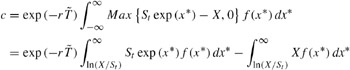
where x* is the risk-neutral variable corresponding to the underlying asset return between now and the maturity of the option. f(x* ) denotes the risk-neutral distribution, which we take to be the normal so that x ^*~ N( r, ? ²). The second integral is easily evaluated whereas the first requires several steps. In the end, one obtains the call option price

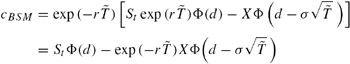
where ? (z) is the cumulative density of a standard normal variable, and where

We will refer to this as the Black-Scholes-Merton (BSM) model. Black, Scholes, and Merton...