6.6. IMPLIED VOLATILITY FUNCTION (IVF) MODELS

The option pricing methods surveyed so far in this chapter can be derived from well-defined assumptions about the underlying dynamics of the economy. The next approach to European option pricing we consider is instead completely static and ad hoc but it turns out to offer reasonably good fit to observed option prices, and we therefore give a brief discussion of it here. The idea behind the approach is that the implied volatility smile changes only slowly over time. If we can therefore estimate a functional form on the smile today, then that functional form may work reasonably in pricing options in the near future as well.

The implied volatility smiles and smirks mentioned earlier suggest that option prices may be well captured by the following four-step approach:

1. Calculate the implied BSM volatilities for all the observed option prices on a given day as

   

2. Regress the implied volatilities on a second-order polynomial in moneyness and maturity. That is, use ordinary least squares (OLS) to estimate the a parameters in the regression

   

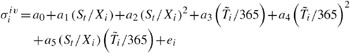
   where e _i is an error term and where we have rescaled maturity to be in years rather than days. The rescaling is done to make the different a coefficients have roughly the same order of magnitude.

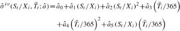
3. Compute the fitted values of implied volatility from the regression,

   

4. Calculate model option prices using the fitted volatilities and the BSM option pricing formula, as in

   

   where the Max(*)...