6.5.1 Formation of W _T

Before moving on to discuss the results, we first examine the weighting matrix used in the stochastic discount factor approach, W _T. Two versions of W _T are calculated. The first version follows the conventional practice and uses excess return in each subsample to obtain W _T at that subsample period. The second version uses the whole sample to create W _T and then uses it as the weighting matrix in each subsample. The reason for using the W _T created from the whole sample is that it is robust to changes in W _T through subsamples and allows us to compare the performance in each model across subsamples.

The prerequisite of calculating the HJ distance is that the weighting matrix, W _T = ( ) ^?1, exists. This requires that the inner product of excess return, , is invertible. We use a measure suggested by Belsley et al. (1980), the condition number, to measure the extent of multicollinearity of . The

condition number is defined by

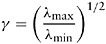
in which ? _max is the largest characteristic root and ? _min is the smallest characteristic root of . For the W _T created by the whole sample, the condition number of ? of the size-sorted portfolios is 12.70 and that of the beta-sorted portfolios ? is 8.39. The invertibility of inner product of excess return in both portfolios seems not to be a problem.