Modelling of Mechanical Systems: Structural Elements, Volume 2

1.3. Hamilton s Principle

1.3. Hamilton s Principle

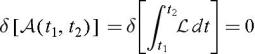
Hamilton s principle has already been introduced and extensively used in [AXI 04] for deriving the Lagrange equations of discrete systems. It is recalled that this variational principle is expressed analytically as:


where ? [] denotes the operator of variation. (t 1, t 2 ) is the action between two arbitrary times t 1 and t 2 of the extended Lagrangian , defined as:


? ([ q], [ ] ) denotes the kinetic energy of the system, p ([ q] ) the internal potential energy, expressed in terms of the generalized displacements and velocity vectors [ q] and [ ]. Q is the work function of extra external or/and internal generalized force vectors [ Q] applied to the system, which are not necessarily conservative. The dimension of all the vectors just mentioned is equal to the number ND of the degrees of freedom (DOF) of the system. Here, Hamilton s principle will be extended to continuous media, providing us with a very efficient analytical tool for dealing with:

  1. the kinematical constraints,

  2. the boundary conditions,

  3. various numerical methods for obtaining approximate solutions of the differential equations of static and dynamic equilibrium.

1.3.1 General presentation of the formalism

The spatial domain occupied by the body and its boundary are still denoted by ( ) and ( ) respectively, though, depending on the dimension of the Euclidean space considered, ( )

UNLIMITED FREE
ACCESS
TO THE WORLD'S BEST IDEAS

SUBMIT
Already a GlobalSpec user? Log in.

This is embarrasing...

An error occurred while processing the form. Please try again in a few minutes.

Customize Your GlobalSpec Experience

Category: Flip-Flops
Finish!
Privacy Policy

This is embarrasing...

An error occurred while processing the form. Please try again in a few minutes.