Overview
The principle of likelihood is based on a probability density function. Although the method is applicable to any form of the density function distribution, for mathematical tractability we consider the Gaussian (normal) distribution, which is completely determined by the mean and covariance matrix. It is the most widely used assumption in practical cases.
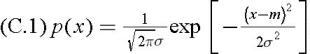
The probability density function of a Gaussian (normally) distributed, scalar real random variable x is given by1 ,2
where m = E{ x} and ? 2 = E{( x ? m) 2} denote the mean value and variance respectively, and E the expected value.
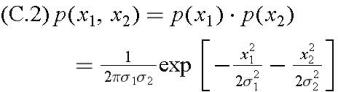
Consider two statistically independent, Gaussian variables x 1 and x 2 with zero mean and variances ? 1 and ? 2, respectively. Then the joint probability density function is given by
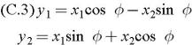
Define two random variables y 1 and y 2, which are obtained from x 1 and x 2 through the rotational transformation
satisfying the condition (  ). Since we assumed that the random variables x 1 and x 2 have zero mean, the mean values of the random variables y 1 and y 2 are also zero. Their variances are given by the expected values of Eq. (C.3):
and the nonzero covariance is given by
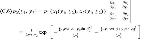
The joint probability density function of y 1 and y 2 is now obtained as
In terms of the second moments of