Effective Maintenance Management: Risk and Reliability Strategies for Optimizing Performance

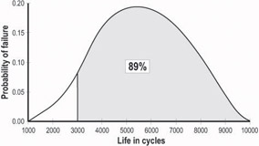
This brings us to the concept of probability density functions. In the earlier example, we can smooth the histogram in Figure 3.1 and obtain a result as seen in Figure 3.2. The area under the curve represents the 37 failures, and is normalized by dividing the number of failures at any point by 37, the sample size. In reliability engineering terminology, we call this normalized curve a probability density function or pdf curve. Since we tested all the items in the sample to destruction, the ratio of the total number of failures to the sample size is 1. The total area under the pdf curve represents the proportion of cumulative failures, which is also 1.
If we draw a vertical line at time t = 3,000 cycles, the height of the curve gives the number of failures as a proportion to the sample size, at this point in time. The area to the left of this line represents the cumulative failure probability of 11%, or the chance that 4 of the 37 items would have failed. The area to the right represents the survival probability of 89%. In reliability engineering terminology, the survival probability is the same as its reliability, and the terms are interchangeable.