5.3 Solutions of Ordinary Differential Equations (ODE)
A function y = f (x) is a solution of a differential equation if the latter is satisfied when y and its derivatives are replaced throughout by f(x) and its corresponding derivatives. Also, the initial conditions must be satisfied.
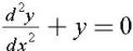
For example a solution of the differential equation
is
since y and its second derivative satisfy the given differential equation.
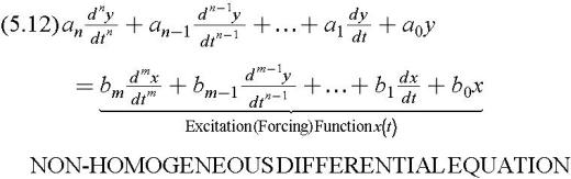
Any linear, time-invariant system can be described by an ODE which has the form
If the excitation in (B12) is not zero, that is, if x(t) ? 0, the ODE is called a non-homogeneous ODE. If x(t) = 0, it reduces to:
The differential equation of (5.13) above is called a homogeneous ODE and has n different linearly independent solutions denoted as y 1(t), y 2(t), y 3(t), , y n(t).
We will now prove that the most general solution of (5.13) is:
where the subscript H on the left side is used to emphasize that this is the form of the solution of the homogeneous ODE and k 1, k 2, k 3, , k n are arbitrary constants.
Proof:
Let us assume that y 1(t) is a solution of (5.13); then by substitution,
A solution of the form k 1y 1(t) will also satisfy (5.13) since
If y = y 1(t) and y = y 2(t) are any two solutions,...


 TABLE OF CONTENTS