Numerical Methods in Engineering with Python

For engineering students and practicing engineers, this text discusses numerical methods thoroughly and illustrates them with problems involving both hand computation and programming.
 TABLE OF CONTENTS
 Given the n+1 data points (x i , y i ), i=0,1,..., n, estimate y(x).
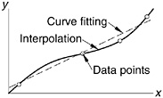
Discrete data sets, or tables of the form are commonly involved in technical calculations. The source of the data may be experimental observations or numerical computations. There is a distinction between interpolation and curve fitting. In interpolation we construct a curve through the data points. In doing so, we make the implicit assumption that the data points are accurate and distinct. Curve fitting is applied to data that contain scatter (noise), usually due to measurement errors. Here we want to find a smooth curve that approximates the data in some sense. Thus the curve does not necessarily hit the data points. The difference between interpolation and curve fitting is illustrated in Fig. 3.1.
| x 0 | x 1 | x 2 |
| x n |
| y 0 | y 1 | y 2 |
| y n |
The simplest form of an interpolant is a polynomial. It is always possible to construct a unique polynomial of degree n that passes through n+1 distinct data points. One means of obtaining this polynomial is the formula of Lagrange
| (3.1a) | 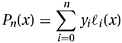 |
where the subscript n denotes the degree of the polynomial and
| (3.1b) | 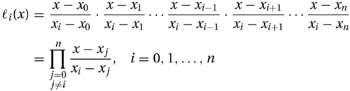 |
are called the cardinal functions.
For example, if n=1, the interpolant is the straight line P 1 (x)=y 0 ? 0 (x)+ y 1 ?