6.2 Classical Stationary Iterative Methods

One of the classical iterative methods is Landweber iteration ^[17], which takes the form

where x ⁽⁰⁾ is the starting vector (often x ⁽⁰⁾ = 0), ? is a real parameter satisfying 0 < ? < 2 ? A ^T A ? ^?1 ₂, and r ^{( k)} = b ? A x ^{( k)} is the residual vector corresponding to x ^{( k)}. This method was generalized by Strand [327] to a scheme of the form

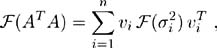
where is a rational function of A ^TA. Classical Landweber iteration thus corresponds to is the SVD of A, then the eigenvalue decomposition of is given by

and it is easy to show that the filter factors f ^{( k)} _i for the kth iteration vector x ^{( k)} in (6.3) are given by

In this way, the iteration number k determines the filter factors and thus it plays the role of a regularization parameter. In particular, the filter factors for (6.2) become

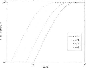
in which case f ^{( k)} _i ? k ?? ² _i for ? _i << ? ^?1/2 while f ^{( k)} _i ? 1 for the large ? _i; cf. [171, 6.1]. See also Fig. 6.1.

Figure 6.1: Plots of the function 1 ? (1 ? ? ? ²)