INTRODUCTION INTRODUCTION
This book discusses mathematical approaches to the best possible way of estimating the state of a general system. Although the book is firmly grounded in mathematical theory, it should not be considered a mathematics text. It is more of an engineering text, or perhaps an applied mathematics text. The approaches that we present for state estimation are all given with the goal of eventual implementation in software.1 The goal of this text is to present state estimation theory in the most clear yet rigorous way possible, while providing enough advanced material and references so that the reader is prepared to contribute new material to the state of the art. Engineers are usually concerned with eventual implementation, and so the material presented is geared toward discrete-time systems. However, continuous-time systems are also discussed for the sake of completeness, and because there is still room for implementations of continuous-time filters. Before we discuss optimal state estimation, we need to define what we mean by the term state. The states of a system are those variables that provide a complete representation of the internal condition or status of the system at a given instant of time.2 This is far from a rigorous definition, but it suffices for the purposes of this introduction. For example, the states of a motor might include the currents through the windings, and the position and speed of the motor shaft. The states of an orbiting satellite might include its position, velocity, and angular orientation. The states of an economic system might include per-capita income, tax rates, unemployment, and economic growth. The states of a biological system might include blood sugar levels, heart and respiration rates, and body temperature. State estimation is applicable to virtually all areas of engineering and science. Any discipline that is concerned with the mathematical modeling of its systems is a likely (perhaps inevitable) candidate for state estimation. This includes electrical engineering, mechanical engineering, chemical engineering, aerospace engineering, robotics, economics, ecology, biology, and many others. The possible applications of state estimation theory are limited only by the engineer's imagination, which is why state estimation has become such a widely researched and applied discipline in the past few decades. State-space theory and state estimation was initially developed in the 1950s and 1960s, and since then there have been a huge number of applications. A few applications are documented in [Sor85]. Thousands of other applications can be discovered by doing an Internet search on the terms "state estimation" and "application," or "Kalman filter" and "application." State estimation is interesting to engineers for at least two reasons: - Often, an engineer needs to estimate the system states in order to implement a state-feedback controller. For example, the electrical engineer needs to estimate the winding currents of a motor in order to control its position. The aerospace engineer needs to estimate the attitude of a satellite in order to control its velocity. The economist needs to estimate economic growth in order to try to control unemployment. The medical doctor needs to estimate blood sugar levels in order to control heart and respiration rates.
- Often an engineer needs to estimate the system states because those states are interesting in their own right. For example, if an engineer wants to measure the health of an engineering system, it may be necessary to estimate the internal condition of the system using a state estimation algorithm. An engineer might want to estimate satellite position in order to more intelligently schedule future satellite activities. An economist might want to estimate economic growth in order to make a political points A medical doctor might want to estimate blood sugar levels in order to evaluate the health of a patient.
There are many other fine books on state estimation that are available (see Appendix B). This begs the question: Why yet another textbook on the topic of state estimation? The reason that this present book has been written is to offer a pedagogical approach and perspective that is not available in other state estimation books. In particular, the hope is that this book will offer the following: - A straightforward, bottom-up approach that assists the reader in obtaining a clear (but theoretically rigorous) understanding of state estimation. This is reminiscent of Gelb's approach [Gel74], which has proven effective for many state estimation students of the past few decades. However, many aspects of Gelb's book have become outdated. In addition, many of the more recent books on state estimation read more like research monographs and are not entirely accessible to the average engineering student. Hence the need for the present book.
- Simple examples that provide the reader with an intuitive understanding of the theory. Many books present state estimation theory and then follow with examples or problems that require a computer for implementation. However, it is possible to present simple examples and problems that require only paper and pencil to solve. These simple problems allow the student to more directly see how the theory works itself out in practice. Again, this is reminiscent of Gelb's approach [Gel74].
- MATLAB-based source code3 for the examples in the book is available at the author's Web site.4 A number of other texts supply source code, but it is often on disk or CD, which makes the code subject to obsolescence. The author's e-mail address is also available on the Web site, and I enthusiastically welcome feedback, comments, suggestions for improvements, and corrections. Of course, Web addresses are also subject to obsolescence, but the book also contains algorithmic, high-level pseudocode listings that will last longer than any specific software listings.
- Careful treatment of advanced topics in optimal state estimation. These topics include unscented filtering, high-order nonlinear filtering, particle filtering, constrained state estimation, reduced-order filtering, robust Kalman filtering, and mixed Kalman/H∞ filtering. Some of these topics are mature, having been introduced in the 1960s, but others of these topics are recent additions to the state of the art. This coverage is not matched in any other books on the topic of state estimation.
Some of the other books on state estimation offer some of the above features, but no other books offer all of these features. Prerequisites The prerequisites for understanding the material in this book are a good foundation in linear systems theory and probability and stochastic processes. Ideally, the reader will already have taken a graduate course in both of these topics. However, it should be said that a background in linear systems theory is more important than probability. The first two chapters of the book review the elements of linear systems and probability that are essential for the rest of the book, and also serve to establish the notation that is used during the remainder of the book. Other material could also be considered prerequisite to understanding this book, such as undergraduate advanced calculus, control theory, and signal processing. However, it would be more accurate to say that the reader will require a moderately high level of mathematical and engineering maturity, rather than trying to identify a list of required prerequisite courses. Problems The problems at the end of each chapter have been written to give a high degree of flexibility to the instructor and student. The problems include both written exercises and computer exercises. The written exercises are intended to strengthen the student's grasp of the theory, and deepen the student's intuitive understanding of the concepts. The computer exercises are intended to help the student learn how to apply the theory to problems of the type that might be encountered in industrial or government projects. Both types of problems are important for the student to become proficient at the material. The distinction between written exercises and computer exercises is more of a fuzzy division rather than a strict division. That is, some of the written exercises include parts for which some computer work might be useful (even required), and some of the computer exercises include parts for which some written analysis might be useful (even required). A solution manual to all of the problems in the text (both written exercises and computer exercises) is available from the publisher to instructors who have adopted this book. Course instructors are encouraged to contact the publisher for further information about out how to obtain the solution manual. Outline of the book This book is divided into four parts. The first part of the book covers introductory material. Chapter 1 is a review of the relevant areas of linear systems. This material is often covered in a first-semester graduate course taken by engineering students. It is advisable, although not strictly required, that readers of this book have already taken a graduate linear systems course. Chapter 2 reviews probability theory and stochastic processes. Again, this is often covered in a first-semester graduate course. In this book we rely less on probability theory than linear systems theory, so a previous course in probability and stochastic processes is not required for the material in this book (although it would be helpful). Chapter 3 covers least squares estimation of constants and Wiener filtering of stochastic processes. The section on Wiener filtering is not required for the remainder of the book, although it is interesting both in its own right and for historical perspective. Chapter 4 is a brief discussion of how the statistical measures of a state (mean and covariance) propagate in time. Chapter 4 provides a bridge from the first, three chapters to the second part of the book. The second part of the book covers Kalman filtering, which is the workhorse of state estimation. In Chapter 5, we derive the discrete-time Kalman filter, including several different (but mathematically equivalent) formulations. In Chapter 6, we present some alternative Kalman filter formulations, including sequential filtering, information filtering, square root filtering, and U-D filtering. In Chapter 7, we discuss some generalizations of the Kalman filter that make the filter applicable to a wider class of problems. These generalizations include correlated process and measurement noise, colored process and measurement noise, steady-state filtering for computational savings, fading-memory filtering, and constrained Kalman filtering. In Chapter 8, we present the continuous-time Kalman filter. This chapter could be skipped if time is short since the continuous-time filter is rarely implemented in practice. In Chapter 9, we discuss optimal smoothing, which is a way to estimate the state of a system at time τ based on measurements that extend beyond time τ. As part of the derivation of the smoothing equations, the first section of Chapter 9 presents another alternative form for the Kalman filter. Chapter 10 presents some additional, more advanced topics in Kalman filtering. These topics include verification of filter performance, estimation in the case of unknown system models, reduced-order filtering, increasing the robustness of the Kalman filter, and filtering in the presence of measurement synchronization errors. This chapter should provide fertile ground for students or engineers who are looking for research topics or projects. The third part of the book covers H∞ filtering. This area is not as mature as Kalman filtering and so there is less material than in the Kalman filtering part of the book. Chapter 11 introduces yet another alternate Kalman filter form as part of the H∞ filter derivation. This chapter discusses both time domain and frequency domain approaches to H∞ filtering. Chapter 12 discusses advanced topics in H∞ filtering, including mixed Kalman/H∞ filtering and constrained H∞ filtering. There is a lot of room for further development in H∞ filtering, and this part of the book could provide a springboard for researchers to make contributions in this area. The fourth part of the book covers filtering for nonlinear systems. Chapter 13 discusses nonlinear filtering based on the Kalman filter, which includes the widely used extended Kalman filter. Chapter 14 covers the unscented Kalman filter, which is a relatively recent development that provides improved performance over the extended Kalman filter. Chapter 15 discusses the particle filter, another recent development that provides a very general solution to the nonlinear filtering problem. It is hoped that this part of the book, especially Chapters 14 and 15, will inspire researchers to make further contributions to these new areas of study. The book concludes with three brief appendices. Appendix A gives some historical perspectives on the development of the Kalman filter, starting with the least squares work of Roger Cotes in the early 1700s, and concluding with the space program applications of Kalman filtering in the 1960s. Appendix B discusses the many other books that have been written on Kalman filtering, including their distinctive contributions. Finally, Appendix C presents some speculations on the connections between optimal state estimation and the meaning of life. Figure I.1 gives a graphical representation of the structure of the book from a prerequisite point of view. For example, Chapter 3 builds on Chapters 1 and 2. Chapter 4 builds on Chapter 3, and Chapter 5 builds on Chapter 4. Chapters 6-11 each depend on material from Chapter 5, but are independent from each other. Chapter 12 builds on Chapter 11. Chapter 13 depends on Chapter 8, and Chapter 14 depends on Chapter 13. Finally, Chapter 15 builds on Chapter 3. This structure can be used to customize a course based on this book. A note on notation Three dots between delimiters (parenthesis, brackets, or braces) means that the quantity between the delimiters is the same as the quantity between the previous set of identical delimiters in the same equation. For example, (A + BCD) + (-..)T = {A + BCD) + (A + BCD)T
A+[B(C + D)]-1E[...]] = A+[B(C + D)]-1E[B(C + D)] (I.1) 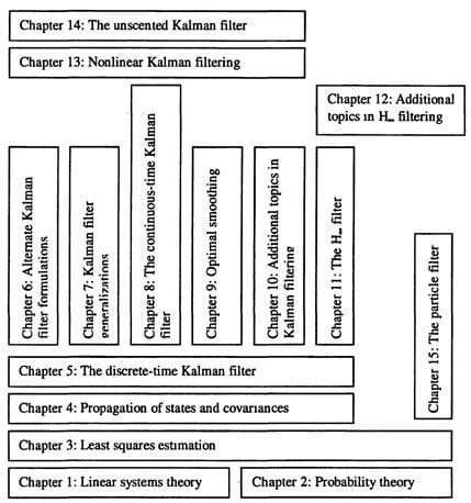 Figure I.1 Prerequisite structure of the chapters in this book. 1I use the practice that is common in academia of referring to a generic third person by the word we. Sometimes, I use the word we to refer to the reader and myself. Other times, I use the word we to indicate that I am speaking on behalf of the control and estimation community. The distinction should be clear from the context. However, I encourage the reader not to read too much into my use of the word we; it is more a matter of personal preference and style rather than a claim to authority. 2In this book, we use the terms state and state variable interchangeably. Also, the word state could refer to the entire collection of state variables, or it could refer to a single state variable. The specific meaning needs to be inferred from the context. 3MATLAB is a registered trademark of The MathWorks, Inc. 4http://academic.csuohio.edu/simond/estimation - if the Web site address changes, it should be easy to find with an internet search. |