|
 INTRODUCTION
Chapter 9.4 - Fixed-Interval Smoothing
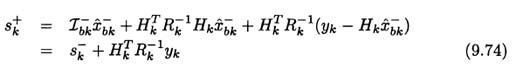
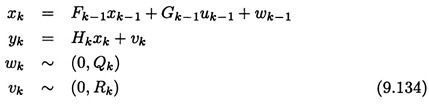
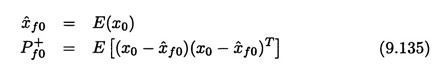
9.4 FIXED-INTERVAL SMOOTHINGSuppose we have measurements for a fixed time interval. In fixed-interval smoothing we seek an estimate of the state at some of the interior points of the time interval. During the smoothing process we do not obtain any new measurements. Section 9.4.1 discusses the forward-backward approach to smoothing, which is perhaps the most straightforward smoothing algorithm. Section 9.4.2 discusses the RTS smoother, which is conceptually more difficult but is computationally cheaper than forward-backward smoothing. 9.4.1 Forward-backward smoothing Suppose we want to estimate the state xmbased on measurements from k = 1 to k = N, where N > m. The forward-backward approach to smoothing obtains two estimates of xm. The first estimate, Suppose that we combine a forward estimate where Kf and Kb are constant matrix coefficients to be determined. Note that The covariance of the estimate can then be found as 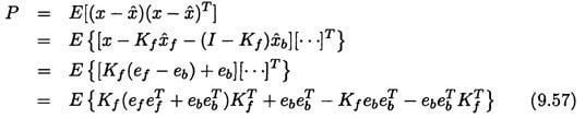 where ef = x - xf , eb = x - xb, and we have used the fact that 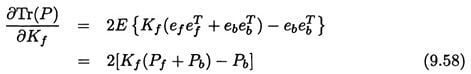 where Pf = 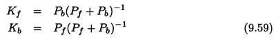 The inverse of (Pf + Pb) always exists since both covariance matrices are positive definite. We can substitute this result into Equation (9.57) to find the covariance of the fixed-interval smoother as follows: 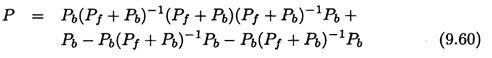 Using the identity (A + B) -1 = B - 1(AB -1 + I) -1 (see Problem 9.2), we can write the above equation as 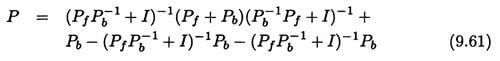 Multiplying out the first term, and again using the identity (A + B) -1 = B - 1(AB -1 + I) -1on the last two terms, results in 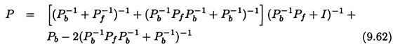 From the matrix inversion lemma of Equation (1.39) we see that Substituting this into Equation (9.62) gives 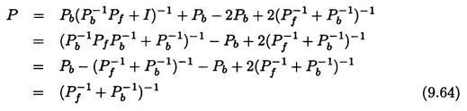 These results form the basis for the fixed-interval smoothing problem. The system model is given as 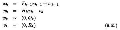 Suppose we want a smoothed estimate at time index m. First we run the forward Kalman filter normally, using measurements up to and including time m.
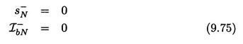
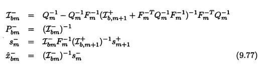
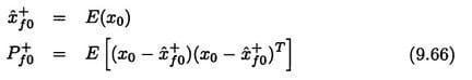 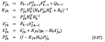 At this point we have a forward estimate for xm, along with its covariance. These quantities are obtained using measurements up to and including time m. The backward filter needs to run backward in time, starting at the final time index N. Since the forward and backward estimates must be independent, none of the information that was used in the forward filter is allowed to be used in the backward filter. Therefore,
We are using the minus superscript on Now the question arises how to initialize the backward state estimate A minus or plus superscript can be added on all the quantities in the above equation to indicate values before or after the measurement at time k is taken into account. Since The infinite boundary condition on 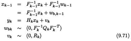 Note that
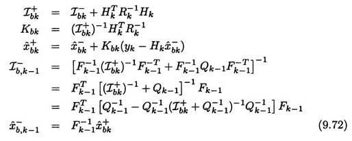 The first form for The third form for Since we need to update sk = 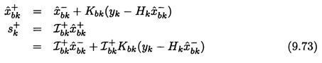 Now note from Equation (6.33) that we can write
We combine this with Equation (9.72) to write the backward information filter as follows.
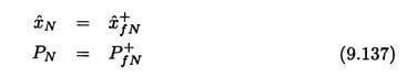
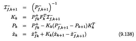
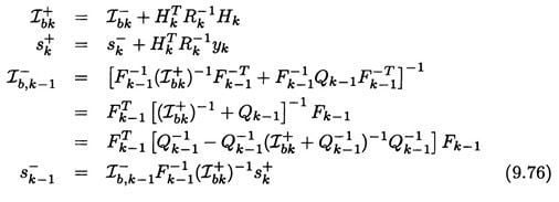  Now we have the backward estimate After we obtain the backward quantities as outlined above, we combine them with the forward quantities from Equation (9.67) to obtain the final state estimate and covariance: 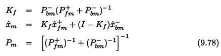 We can obtain an alternative equation for 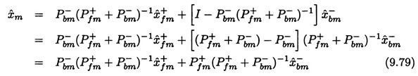 Using the matrix inversion lemma on the rightmost inverse in the above equation and performing some other manipulations gives 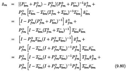 where we have relied on the identity(A + B) -1 = B - 1(AB -1 + I) -1 (see Problem 9.2). The coefficients of 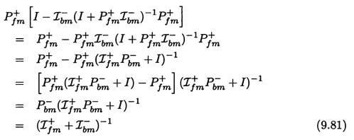 Therefore, using Equation (9.78), we can write Equation (9.80) as 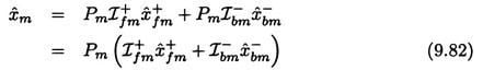 Figure 9.9 illustrates how the forward-backward smoother works.  Figure 9.9 This figure illustrates the concept of the forward-backward smoother. The forward filter is run to obtain a posteriori estimates and covariances up to time m. Then the backward filter is run to obtain a priori estimates and covariances back to time m (i.e., a priori from a reversed time perspective). Then the forward and backward estimates and covariances at time m are combined to obtain the final estimate ■ EXAMPLE 9.3 In this example we consider the same problem given in Example 9.1. Suppose that we want to estimate the position and velocity of the vehicle at t = 5 seconds. We have measurements every 0.1 seconds for a total of 10 seconds. The standard deviation of the measurement noise is 10, and the standard deviation of the acceleration noise is 10. Figure 9.10 shows the trace of the covariance of the estimation of the forward filter as it runs from t = 0 to t = 5, the backward filter as it runs from t = 10 back to t = 5, and the smoothed estimate at t = 5. The forward and backward filters both converge to the same steady-state value, even though the forward filter was initialized to a covariance of 20 for both the position and velocity estimation errors, and the backward filter was initialized to an infinite covariance. The smoothed filter has a covariance of about 7.6, which shows the dramatic improvement that can be obtained in estimation accuracy when smoothing is used. 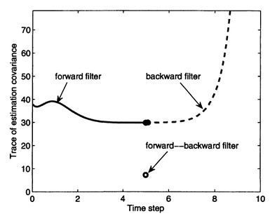 Figure 9.10 This shows the trace of the estimation-error covariance for Example 9.3. The forward filter runs from 9.4.2 RTS smoothing Several other forms of the fixed-interval smoother have been obtained. One of the most common is the smoother that was presented by Rauch, Tung, and Striebet, usually called the RTS smoother [Rau65]. The RTS smoother is more computationally efficient than the smoother presented in the previous section because we do not need to directly compute the backward estimate or covariance in order to get the smoothed estimate and covariance. In order to obtain the RTS smoother, we will first look at the smoothed covariance given in Equation (9.78) and obtain an equivalent expression that does not use Pbm. Then we will look at the snoothed estimate given in Equation (9.78), which uses the gain Kf, which depends on Pbm, and obtain an equivalent expression that does not use Pbm or 9.4.2.1 RTS covariance updateFirst consider the smoothed covariance given in Equation (9.78). This can be written as 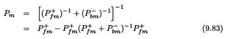 where the second expression comes from an application of the matrix inversion lemma to the first expression (see Problem 9.3). Prom Equation (9.72) we see that 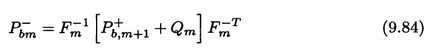 Substituting this into the expression ( 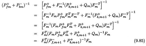 From Equations (6.26) and (9.76) recall that 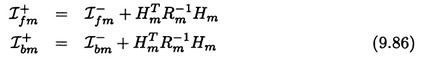 We can combine these two equations to obtain Substituting this into Equation (9.78) gives 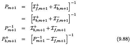 Substituting this into Equation (9.85) gives 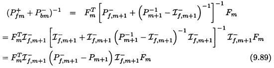 where the last equality comes from an application of the matrix inversion lemma. Substituting this expression into Equation (9.83) gives where the smoother gain Kmis given as The covariance update equation for Pm is not a function of the backward covariance. The smoother covariance Pmcan be solved by using only the forward covariance Pfm , which reduces the computational effort (compared to the algorithm presented in Section 9.4.1). 9.4.2.2 RTS state estimate updateNext we consider the smoothed estimate Lemma 1 Proof: From Equation (9.67) we see that Rearranging this equation gives Premultiplying both sides by Lemma 2The a posteriori covariance Proof: From Equation (9.78) we obtain 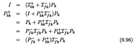 QED Lemma 3The covariances of the forward and backward filters satisfy the equation Proof: From Equation (9.67) and (9.72) we see that 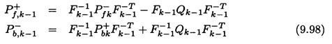 Adding these two equations and rearranging gives 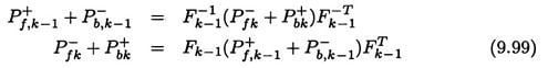 QED Lemma 4The smoothed estimate Proof: From Equations (9.69) and (9.82) we have 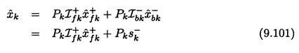 From Equation (9.76) we see that Substitute this expression for Now substitute 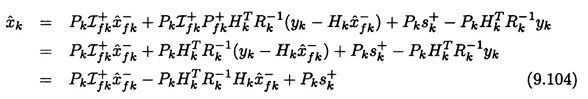 QED Lemma 5 Proof: Recall from Equations (6.26) and (9.72) that 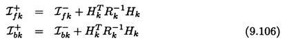 Combining these two equations gives 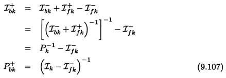 where we have used Equation (9.78) in the above derivation. Substitute this expression for 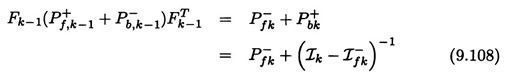 Invert both sides to obtain 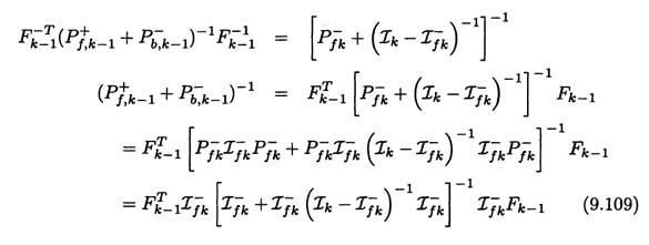 Now apply the matrix inversion lemma to the term 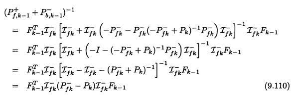 QED With the above lemmas we now have the tools that we need to obtain an alternate expression for the smoothed estimate. Starting with the expression for 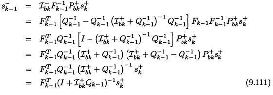 Rearranging this equation gives Multiplying out this equation, and premultiplying both sides by Substituting for 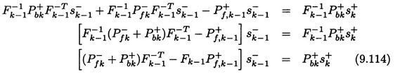 Substituting in this expression for
Substituting for 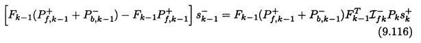 Premultiplying both sides by  Substituting Equation (9.105) for Now from Equation (9.105) we see that So we can add the two sides of this equation to the two sides of Equation (9.118) to get  Now use Equation (9.100) to substitute for Pk 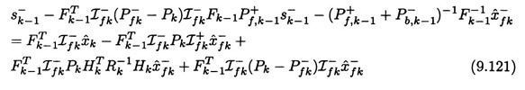 Rearrange this equation to obtain 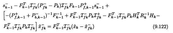 From Equation (9.106) we see that From Equation (9.67) we see that  Now substitute for Pkfrom Equation (9.90) and use Equation (9.91) in the above equation to obtain
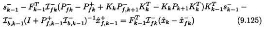
Premultiplying both sides by  Now use Equation (9.91) to notice that the coefficient of Using Equation (9.90) to substitute for 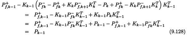 Since this is the coefficient of Now from Equations (9.78) and (9.82) we see that 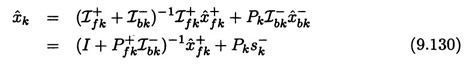 From this we see that 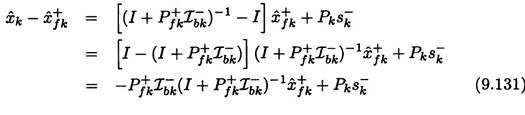 Rewriting the above equation with the time subscripts (k - 1) and then substituting for the left side of Equation (9.129) gives from which we can write This gives the smoothed estimate The RTS smoother
     |
 is the covariance of the forward estimate, and Pb =
  is the covariance of the backward estimate. Setting this equal to zero to find the optimal value of Kfgives