|
 INTRODUCTION
Chapter 9.2 - Fixed-Point Smoothing
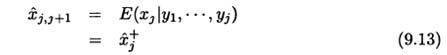
9.2 FIXED-POINT SMOOTHINGThe objective in fixed-point smoothing is to obtain a priori state estimates of xj at times j + 1, j + 2, …, k, k + 1, …. We will use the notation With this definition we see that 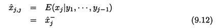 In other words,
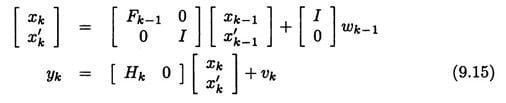
 In order to derive the fixed-point smoother, we will define a new state variable x'. This new state variable will be initialized as x'j = xj, and will have the dynamics x'k+1= x'k (k = j, j +1,…). With this definition, we see that Our original system is given as 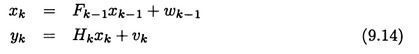
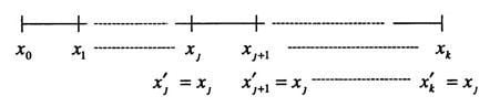
Figure 9.4 This illustrates the idea that is used to obtain the fixed-point smoother. A fictitious state variablex' is initialized asx'j= xj and from that point on has an identity-state transition matrix. The a priori estimate of x'kis then equal to Augmenting the dynamics of our newly defined statex' to the original system results in the following:
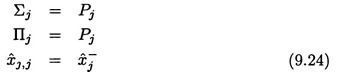
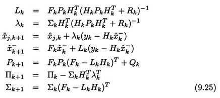
If we use a standard Kalman filter to obtain an a priori estimate of the augmented state, the covariance of the estimation error can be written as  The covariance Pk above is the normal a priori covariance of the estimate of xk. We have dropped the minus superscript for ease of notation, and we will also feel free to drop the minus superscript on all other quantities in this section with the understanding that all estimates and covariances are a priori. The Σk and Πk matrices are defined by the above equation. Note that at time k= j, Σk and Πk are given as 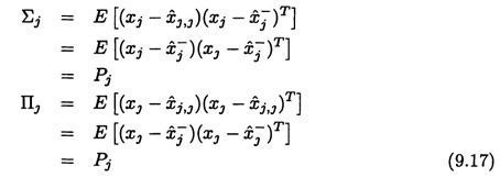 The Kalman filter summarized in Equation (9.10) can be written for the augmented system as follows:  where Lk is the normal Kalman filter gain given in Equation (9.10), and λk is the additional part of the Kalman gain, which will be determined later in this section. Writing Equation (9.18) as two separate equations gives 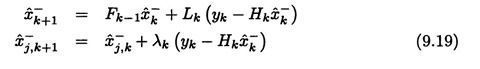 The Kalman gain can be written from Equation (9.10) as follows: 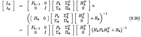 Writing this equation as two separate equations gives  The Kalman filter estimation-error covariance-update equation can be written from Equation (9.10) as follows: 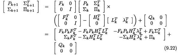 Writing this equation as three separate equations gives 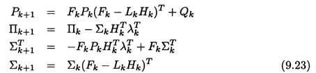 It is not immediately apparent from the above expressions that Equations (9.19) - (9.23) completely define the fixed-point smoother. The fixed-point smoother, which is used for obtaining The fixed-point smoother
As we recall from Equation (9.16), Pkis the a priori covariance of the standard Kalman filter estimate, Πk is the covariance of the smoothed estimate of xj at time k, and Σk is the cross covariance between the two. 9.2.1 Estimation improvement due to smoothing Now we will look at the improvement in the estimate of xj due to smoothing. The estimate  Now assume for purposes of additional analysis that the system is time-invariant and the covariance of the standard filter has reached steady state at time j. Then we have From Equation (9.25) we see that where Σ is initialized as Σj = P. Combining this expression for Σk+1 with its initial value, we see that 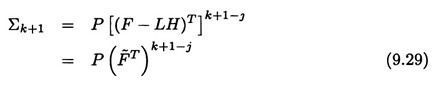 where 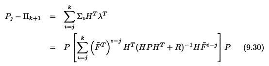 The quantity on the right side of this equation is positive definite, which shows that the smoothed estimate of xj is always better than the standard Kalman filter estimate. In other words, (Pj - Πk+1) > 0, which implies that Πk+1< Pj. Furthermore, the quantity on the right side is a sum of positive definite matrices, which shows that the larger the value of k (i.e., the more measurements that we use to obtain our smoothed estimate), the greater the improvement in the estimation accuracy. Also note from the above that the quantity (HPHT + R) inside the summation is inverted. This shows that as R increases, the quantity on the right side decreases. In the limit we see from Equation (9.30) that This illustrates the general principle that the larger the measurement noise, the smaller the improvement in estimation accuracy that we can obtain by smoothing. This is intuitive because large measurement noise means that additional measurements will not provide much improvement to our estimation accuracy. ■ EXAMPLE 9.1 In this example, we will see the improvement due to smoothing that can be obtained for a vehicle navigation problem. This is a second-order Newtonian system where x(1) is position and x(2) is velocity. The input is comprised of a commanded acceleration u plus acceleration noise 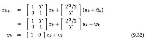 Note that the process noise wkis given as  Now suppose the acceleration noise  The percent improvement due to smoothing can be defined as  where j is the point which is being smoothed, and k is the number of measurements that are processed by the smoother. We can run the fixed-point smoother given by Equation (9.25) in order to smooth the position and velocity estimate at any desired time. Suppose we use the smoother equations to smooth the estimate at the second time step (k = 1). If we use measurements at times up to and including 10 seconds to estimate x1, then our estimate is denoted as Table 9.1 Improvement due to smoothing the state at the first time step after 10 seconds for Example 9.1. The improvement due to smoothing is more noticeable when the measurement noise is small.  Figure 9.5 shows the trace of Πk, which is the covariance of the estimation error of the state at the first time step. As time progresses, our estimate of the state at the first time step improves. After 10 seconds of additional measurements, the estimate of the state at the first time step has improved by 96.6% relative to the standard Kalman filter estimate. Figure 9.6 shows the smoothed estimation error of the position and velocity of the first time step. We see that processing more measurements decreases the estimation-error covariance. In general, the smoothed estimation errors shown in Figure 9.6 will converge to nonzero values. The estimation errors are zero-mean, but not for  Figure 9.5 This shows the trace of the estimation-error covariance of the smoothed estimate of the state at the first time step for Example 9.1. As time progresses and we process more measurements, the covariance decreases, eventually reaching steady state.  Figure 9.6 This shows typical estimation errors of the smoothed estimate of the state at the first time step for Example 9.1. As time progresses and we process more measurements, the estimation error decreases, and its standard deviation eventually reaches steady state. any particular simulation. The estimation errors are zero-mean when averaged over many simulations. The system discussed here was simulated 1000 times and the variance of the estimation errors (x1 - 9.2.2 Smoothing constant states Now we will think about the improvement (due to smoothing) in the estimation accuracy of constant states. If the system states are constant then Fk - I and Q = 0. Equation (9.25) shows that  Comparing these expressions for Pk+1 and Σk+1, and realizing from Equation (9.24) that the initial value of Σj = Pk, we see that Σj = Pk for k ≥ j. This means that the expression for Lkfrom Equation (9.25) can be written as  Substituting these results into the expression for Πk+1 from Equation (9.25) we see that  Realizing that the initial value of Πj = Pj, and comparing this expression for Πk+1 with Equation (9.36) for Pk+1, we see that Πk = Pk for k ≥ j. Recall that Pk is the covariance of the estimate of xkfrom the standard Kalman filter, and Πk is the covariance of the estimate of xj given measurements up to and including time (k-1). This result shows that constant states are not smoothable. Additional measurements are still helpful for refining an estimate of a constant state. However, there is no point to using smoothing for estimation of a constant state. If we want to estimate a constant state at time j using measurements up to time k > j, then we may as well simply run the standard Kalman filter up to time k. Implementing the smoothing equations will not gain any improvement in estimation accuracy. |