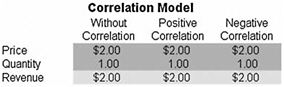
Although the computations required to correlate variables in a simulation are complex, the resulting effects are fairly clear. Figure 4-16 shows a simple correlation model (Correlation Risk Effects Model in the example folder). The calculation for revenue is simply price multiplied by quantity. The same model is replicated for no correlations, positive correlation (+0.9), and negative correlation ( ?0.9) between price and quantity.

Figure 4-16: Simple correlation model.

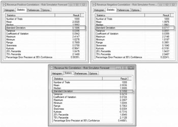
The resulting statistics are shown in Figure 4-17. Notice that the standard deviation of the model without correlations is 0.1450, compared to 0.1886 for the positive cor- relation and 0.0717 for the negative correlation; that is, for simple models with positive relationships (e.g., additions and multiplications), negative correlations tend to reduce the average spread of the distribution and create a tighter and more concentrated forecast distribution as compared to positive correlations with larger average spreads. However, the mean remains relatively stable. This implies that correlations do little to change the expected value of projects but can reduce or increase a portfo-lio s risk. Recall in financial theory that negatively correlated variables, projects, or assets when combined in a portfolio tend to create a diversification effect where the overall risk is reduced. Therefore, we see a smaller standard deviation for the negatively correlated model.

Figure 4-17: Correlation results.

In a positively related model (e.g., A + B = C or A B = C), a negative correlation reduces the risk (standard deviation...