1. Problem Definition

Defining boundary-value problems for ODEs is different from doing so for the Cauchy problems considered in the previous chapters, in that boundary conditions are specified not for one starting point, but for both ends of the computation interval.

Let s take a system of N first-order ODEs:

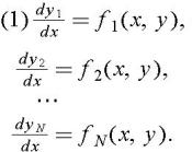
Additionally, some of the N additional conditions are specified for one end of the interval, and the rest of the conditions are specified for the opposite end:

This circumstance is the reason why they are called not initial (as in Cauchy problems), but boundary conditions.

Despite the seeming similarity of boundary-value problems for ODE and Cauchy problems (see Chapters 3 and 4), substantially different computer methods are used for solving them. The finite difference algorithms for solving Cauchy problems can be classified as the recurrence relations between n-th and ( n+1)-th steps (running count). With these methods, the unknown function values for grid points are calculated starting from the known initial conditions by simply using the values already calculated for previous points.

This is not the case with boundary-value problems. Difference equations approximating the ODE represent that the unknown values y(x) in the grid points are linked through a system of linear, or even nonlinear (if the ODE system is itself nonlinear), algebraic equations. Solving it numerically is a separate, sometimes quite difficult (in the case of a nonlinear system), problem.

We will consider two approaches to solving boundary-value problems using the computer.