Chapter List

Overview

In this chapter and the next two we will consider an ordinary differential equation (ODE) system with m components,

subject to m two-point boundary conditions

We denote the Jacobian matrices of g( u, v) with respect to its first and second argument vectors by

Often in applications, g is linear; i.e., the boundary conditions can be written as

for some given data b, ^[25] and the m m matrices B ₀ and B _b are constant.

Also, often in applications the boundary conditions are separated; i.e., each of the components of g is given either at t = 0 or at t = b, but none involves both ends simultaneously. ^[26] In this case for each i, 1 ? i ? m, either the ith row of B ₀ or the ith row of B _b are identically zero.

Example 6.1

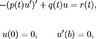
Recall Example 1.4 (the vibrating spring),

where p( t) > 0, q( t) ? 0 for all 0 ? t ? b. In more independent variables, a problem like this corresponds to an elliptic partial differential equation.

To convert this into a system we have two popular options.

• The standard option is to set