3.8 Graphical Analysis

The operation of a simple transistor circuit can also be described graphically. We will use the circuit of Figure 3.42 for our graphical analysis.

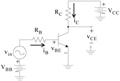Figure 3.42: Circuit showing the variables used on the graphs of Figures 3.43 and 3.44

We start with a plot of i _B versus v _BE to determine the point where the curve

(3.40)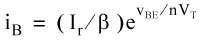

and the equation of the straight line intersect

(3.41)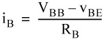

The equation of (3.41) was obtained with the AC source v _in shorted out. This equation can be expressed as

(3.42)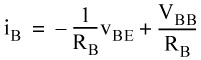

We recognize (3.42) as the equation of a straight line of the form y = mx + b with slope -1/R _B. This equation and the curve of equation (3.40) are shown in Figure 3.43.

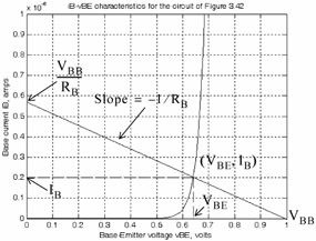Figure 3.43: Plot showing the intersection of Equations (3.40) and (3.42)

We used the following MATLAB script to plot the curve of equation (3.40).

vBE=0: 0.01: 1; iR=10^(-15); beta = 100; n=1; VT=27 ^?10^(-3);...

iB=(iR./beta). ^?exp(vBE./(n.*VT)); plot(vBE,iB); axis([0 1 0 10^(-6)]);...

xlabel('Base-Emitter voltage vBE, volts'); ylabel('Base current iB, amps');...

title('iB-vBE characteristics for the circuit of Figure 3.42'); grid

From Figure 3.43 we obtain the values of V _BE and I _B on the v _BE and i _B axes respectively. Next, we refer to the family of curves of the collector current i _C versus collector-emitter voltage v _CE for different values of i _B as shown in Figure 3.44. where...