International Journal of Numerical Methods for Heat & Fluid Flow: Numerical Methods in Aerospace: Civil Aviation and Space Exploration, Volume 14, Number 4, 2004

A finite-volume Euler code is used for the aerodynamic model. The two-dimensional unsteady Euler equations on a moving grid in integral form are:
| (12) | |
where U is the vector of conserved variables, F is the flux vector, n is the outward cell face unit normal, and S the peripheral length of the cell face. U and F are given by:
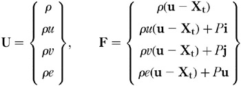
| (13) | |
where u is the velocity vector, X t the grid velocity vector, and P, ?, u, v and e are pressure, density, Cartesian x- and y-component velocities and total specific energy, respectively. The equation set is closed by
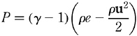
| (14) | |
The unsteady Euler equations are solved using a Jameson (Jameson et al., 1981) type cell-centred finite-volume method. Equation (12) is applied to each cell of the mesh. Following Jameson et al. (1981), the spatial and time dependent terms are decoupled and a set of ordinary differential equations are obtained. Artificial dissipation needs to be added to stabilise the solution (Jameson et al., 1981; Kroll and Jain, 1987).
It is expensive to use explicit time-stepping for unsteady flows. To maintain time-accuracy the whole domain must be integrated by the same time-step, and this is limited to the smallest value over the domain. Hence, an implicit scheme is used, based on that proposed by Jameson (1991). This solves the unsteady flows as a series of pseudo-steady cases,...