Overview

Our starting point is a basic question. Given a set of grid points { x _j} and corresponding function values { u( x _j)}, how can we use this data to approximate the derivative of u? Probably the method that immediately springs to mind is some kind of finite difference formula. It is through finite differences that we shall motivate spectral methods.

To be specific, consider a uniform grid { x ₁, , x _N}, with x _{j + 1} ? x _j = h for each j, and a set of corresponding data values { u ₁, , u _N}:

Let W _j denote the approximation to u ? ( x _j), the derivative of u at x _j. The standard second-order finite difference approximation is

which can be derived by considering the Taylor expansions of U( x _{j + 1}) and u( x _{j ? 1}). For simplicity, let us assume that the problem is periodic and take u ₀ = u _N and u ₁ = u _{N + 1}. Then we can represent the discrete differentiation process as a matrix-vector multiplication,

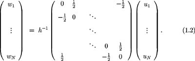
(Omitted entries here and in other sparse matrices in this book are zero.) Observe that this matrix is Toeplitz, having constant entries along diagonals; i.e., a _ij depends only on i ?