Overview

In this chapter we will see how Chebyshev spectral methods can be implemented by the FFT, which provides a crucial speedup for some calculations. Equally important will be the mathematical idea that underlies this technique: the equivalence of

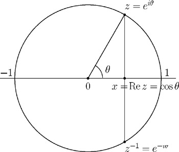
The basis of our development is summarized in Figure 8.1. Let z be a complex number on the unit circle: z = 1. Let ? be the argument of z, a real number that is determined up to multiples of 2 ?. Let x = Re z = cos ?. For each x 2 ? [ ?1, 1], there are two complex conjugate values of z, and we have

The nth Chebyshev polynomial, denoted T _n, is defined by

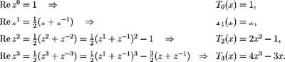
From this formula, it is not obvious that T _n( x) is a polynomial in x. The cases n = 0, 1, 2, and 3 make the point clear:

Figure 8.1: Relationships between x, z, and ?.

In general,

which amounts to the recurrence relation

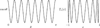
By induction, we deduce that T _n is a polynomial of degree exactly n for each n ? 0, with leading coefficient 2 ^{n ?1} for each n ? 1. Figure 8.2 gives a geometric interpretation.

Figure 8.2: The Chebyshev polynomial T _n can be interpreted as a sine wave "wrapped around a cylinder and viewed from...