Overview

Of course, not all problems can be treated as periodic. We now begin to consider how to construct spectral methods for bounded, nonperiodic domains.

Suppose that we wish to work on [ ?1, 1] with nonperiodic functions. One approach would be to pretend that the functions were periodic and use trigonometric (that is, Fourier) interpolation in equispaced points. This is what we did in Program 8. It is a method that works fine for problems like that one whose solutions are exponentially close to zero (or a constant) near the boundaries. In general, however, this approach sacrifices the accuracy advantages of spectral methods. A smooth function

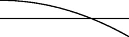
becomes nonsmooth in general when periodically extended:

With a Fourier spectral method, the contamination caused by these discontinuities will be global, destroying the spectral accuracy the Gibbs phenomenon visible in Output 3 (p. 14). The error in the interpolant will be O(1), the error in the first derivative will be O(N), and so on. These errors will remain significant even if extra steps are taken to make the functions under study periodic. To achieve good accuracy by a method of that kind it would be necessary to enforce continuity not just of function values but also of several derivatives (see Theorem 4(a), p. 34), a process neither elegant nor efficient.

Instead, it is customary to replace trigonometric polynomials by algebraic polynomials, p( x) = a ₀ + a ₁ x + + a _Nx