An advantage to building a complex system from simple components by using a few control principles is that complexity is reduced by decomposition. In normal cases it is also comparatively easy to extrapolate the experience of commissioning and tuning single-loop control. It is also appealing to build up a complex system by gradual refinement. There are, however, also some drawbacks with the approach:

• Since we have not determined the fundamental limitations, it is difficult to decide when further refinements do not give any significant benefits.
• It is easy to get systems that are unnecessarily complicated. We may get systems where several control loops are fighting each other.
• There are cases where it is difficult to arrive at a good overall system by a loop-by-loop approach.

If there are difficulties, it is necessary to use a systematic approach based on mathematical modeling analysis and simulation. This is, however, more demanding than the empirical approach. In this section we illustrate some of the difficulties that may arise.

Parallel Systems

Systems that are connected in parallel are quite common. Typical examples are motors that are driving the same load, power systems and networks for steam distribution. Control of such systems require special consideration. To illustrate the difficulties that may arise we will consider the situation with two motors driving the same load. A schematic diagram of the system is shown in Figure 7.27.

Let ? be the angular velocity of the shaft, J the total moment of inertia, and D the damping coefficient. The system can then be described by the equation

where M₁ and M₂ are the torques from the motors and M_l is the load torque.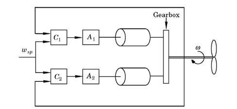

Figure 7.27 Schematic diagram of two motors that drive the same load.

7.8.2 Proportional Control

Assume each motor is provided with a proportional controller. The control strategies are then

In these equations the parameters M₁₀ and M₂₀ give the torques provided by each motor when ? = ?_sp and K₁ and K₂ are the controller gains. It follows from Equations (7.12) and (7.13) that

The closed-loop system is, thus, a dynamical system of first order. After perturbations the angular velocity reaches its steady state with a time constant

The response speed is thus given by the sum of the damping and the controller gains. The stationary value of the angular velocity is given by

This implies that there normally will be a steady state error. Similarly we find from Equation (7.13) that

The ratio of the controller gains will indicate how the load is shared between the motors.

Proportional and Integral Control

The standard way to eliminate a steady state error is to introduce integral action. In Figure 7.28 we show a simulation of the system in which the motors have identical PI controllers. The setpoint is changed at time 0. A load disturbance in the form of a step in the load torque is introduced at time 10 and a pulse-like measurement disturbance in the second motor controller is introduced at time 20. When the measurement error occurs the balance of the torques is changed so that the first motor takes up much more of the load after the disturbance. In this particular case the second motor is actually breaking. This is highly undesirable, of course.

To understand the phenomena we show the block diagram of the system in Figure 7.29. The figure shows that there are two parallel

Figure 7.28 Simulation of a system with two motors with PI controllers that drive the same load. The figure shows setpoint ?sp, process output ?, control signals M₁ and M₂, load disturbance M_L, and measurement disturbance n.

paths in the system that contain integration. This is a standard case where observability and controllability is lost. Expressed differently, it is not possible to change the signals M₁ and M₂ individually from the error. Since the uncontrollable state is an integrator, it does not go to zero after disturbance. This means that the torques can take on arbitrary values after disturbance. For example, it may happen that one of the motors takes practically all the load, clearly an undesirable situation.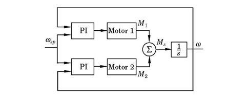

Figure 7.29 Block diagram for the system in Figure 7.28.

Figure 7.30 Block diagram of an improved control system.

7.8.3 How to Avoid the Difficulties

Having understood the reason for the difficulty, it is easy to modify the controller as shown in Figure 7.30. In this case only one controller with integral action is used. The output of this drives proportional controllers for each motor. A simulation of such a system is shown in Figure 7.31. The difficulties are clearly eliminated.

The difficulties shown in the examples with two motors driving the same load are even more accentuated if there are more motors.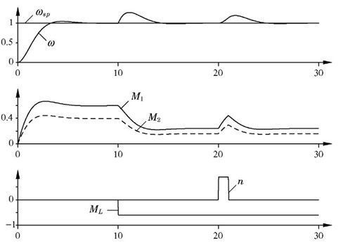

Figure 7.31 Simulation of the system with the modified controller. The figure shows setpoint ?sp, process output ?, control signals M₁ and M₂, load disturbance M_L, and measurement disturbance n.

Good control in this case can be obtained by using one PI controller and distributing the outputs of this PI controller to the different motors, each of which has a proportional controller. An alternative is to provide one motor with a PI controller and let the other have proportional control. To summarize, we have found that there may be difficulties with parallel systems having integral action. The difficulties are caused by the parallel connection of integrators that produce unstable subsystems that are neither controllable nor observable. With disturbances these modes can change in an arbitrary manner. The remedy is to change the control strategies so there is only one integrator.

7.8.4 Interaction of Simple Loops

There are processes that have many control variables and many measured variables. Such systems are called multi-input multi-output (MIMO) systems. Because of the interaction between the signals, it may be very difficult to control such systems by a combination of simple controllers. A reasonably complete treatment of this problem is far outside the scope of this book. Let it suffice to illustrate some difficulties that may arise by considering processes with two inputs and two outputs. A block diagram of such a system is shown in Figure 7.32. A simple approach to control such a system is to use two single-loop controllers, one for each loop. To do this we must first decide how the controllers should be connected, i.e., if y₁ in the figure should be controlled by u₁ or u₂. This is called the pairing problem. This problem is straightforward if there is little interaction among the loops, which can be determined from the responses of all outputs to all inputs (see e.g. Figure 7.33). The single-loop approach will work well if there is small coupling between the loops. The loops can then be tuned separately. There may be difficulties, however, when there is coupling between the loops (as shown in the following example).

Figure 7.32 Block diagram of a system with two inputs and two outputs.

EXAMPLE 7.8 Rosenbrock's system

Consider a system with two inputs and two outputs. Sych a system can be characterized by giving the transfer functions that relate all inputs and outputs. These transfer functions can be organized as the matrix

The first index refers to the outputs and the second to the inputs. In the matrix above, the transfer function gi2 denotes the transfer function from the second input to the first output.

The behavior of the system can be illustrated by plotting the step responses from all inputs, as shown in Figure 7.33. From this figure we can see that there are significant interactions between the signals. The dynamics of all responses do, however, appear quite benign. In this case it is not obvious how the signals should be paired. Arbitrarily, we use the pattern 1-1, 2-2. It is very easy to design a controller for the individual loops if there is no interaction. The transfer function of the process is

in both cases. With PI control it is possible to obtain arbitrarily high gains, if there are no constraints on measurement noise or process uncertainty. A reasonable choice is to have K = 19, b = 0, and T_i = 0.19. This gives a system with relative damping ? = 0.7 and an undamped natural frequency of 10 rad/s. The responses obtained with this controller in one loop and the other loop open are shown in

Figure 7.33 Open-loop step responses of the system. The left diagrams show responses to a step change in control signal u₁ and the right diagrams show responses to a step change in control signal u₂.

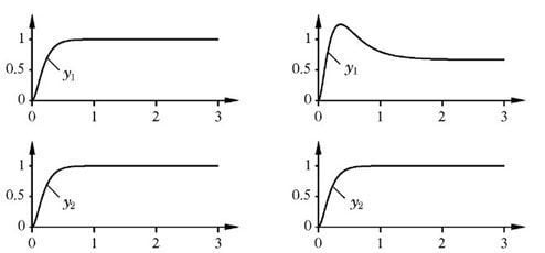Figure 7.34 Step responses with one loop closed and the other open. The left diagrams show responses to steps in u₁ when controller C₂ is disconnected, and the right diagrams show responses to steps in u₂ when controller C₁ is disconnected.

Figure 7.34. Notice that the desired responses are as expected, but that there also are strong responses in the other signals. If both loops are closed with the controllers obtained, the system will be unstable.

In order to have reasonable responses with both loops closed, it is necessary to detune the loops significantly. In Figure 7.35 we show responses obtained when the controller in the first loop has parameters K = 2 and T_i = 0.5 and the other controller has K = 0.8 and T_i = 0.7. The gains are more than an order of magnitude smaller than the ones obtained with one loop open. A comparison with Figure 7.34 shows that the responses are significantly slower.

The example clearly demonstrates the deficiencies in loop-by loop

Figure 7.35 Step responses when both loops are closed. The figure shows responses to simultaneous setpoint changes in both loops.

tuning. The example chosen is admittedly somewhat extreme but it clearly indicates that it is necessary to have other techniques for truly multivariable systems. The reason for the difficulty is that the seemingly innocent system is actually a non-minimum phase multivariable system with a zero at s = -1.

7.8.5 Interaction Measures

The example given clearly indicates the need to have some way to find out if interactions may cause difficulties. There are no simple universal methods. An indication can be obtained by the relative gain array (RGA). This can be computed from the static gains in all loops in a multivariable system. For the a 2 x 2 system like the one in Example 7.8 the RGA is

The number ? has physical interpretation as the ratio of the gain from u₁ to y₁ with the second loop open and with the second loop under very tight feedback (y₂ = 0). There is no interaction if ? = 1. If ? = 0 there is also no interaction, but the loops should be interchanged. The loops should be interchanged when ? < 0.5. The interaction is most severe if ? = 0.5.

For a multivariable system the relative gain is a matrix R in which component r_ij is given by

where g_ij is ij-th element of the static gain matrix G of the process and hij is the ij-th element of the the matrix

Notice that g_ij is the static gain from input j to output i.

Bristol's recommendation for controller pairing is that the measured values and control variables should be paired so that the corresponding relative gains are positive, and as close to one as possible. If the gains are outside the interval 0.67 < ? < 1.5, decoupling can improve the control significantly. Since the relative gain is based on the static properties of the system, it does not capture all aspects of the interaction.