7.2.1 Locally integrable functions and regular distributions

Let us start with deterministic and real functions of time f ( t). By definition, such functions connect to each other the real numbers t ₁ and f ( t ₁), where t ₁ lies within the range of definition of f ( t). Moreover, the mapping t ₁ ? f ( t ₁) is deterministic, which means free of any uncertainty, or randomness. Restricting study to the physical context of mechanics, f ( t) is assumed to be a continuous or a piecewise continuous function of finite magnitude:

(7.2)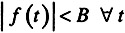

Bounded functions with a finite number of jumps are locally integrable, which means that:

(7.3)

Such functions generate regular distributions defined by the integrals:

(7.4)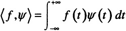

where use is made of the functional vector notation <, > of the scalar product. Accordingly, f( t) and ?( t) are interpreted here as functional vectors, as detailed in Appendix 1. On the other hand, ?( t) designates an auxiliary function, termed test function that complies with the following very restrictive conditions:

• ? ( t) is identically zero, outside a finite interval ?.

• ?( t) can be differentiated up to any desired order.

NOTE. - Theory of distributions

The concept of distributions, introduced first by Dirac, and then formalized mathematically by Schwartz, is a convenient tool for analysing mechanical systems. Appendix...