Modelling of Mechanical Systems: Discrete Systems, Volume 1
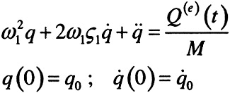
The system [7.1] reduced to a single equation and provided with given initial conditions is written as:
| (7.17) | ![]() |
According to the general theory of linear differential equations, solution of the problem [7.17] can be obtained by adding a special solution of the inhomogeneous differential equation to the general solution of the corresponding homogeneous one. Constants of integration are calculated afterwards in order to fit the initial conditions of the specific problem to be treated. However, for a systematic study of the solutions, where the exciting signal is varied at will, it is found preferable to make use of the Laplace transform technique. As we will see in the next subsection, obtaining the Laplace transform of the solution is an easy task, producing quite valuable information on the physical problem. Then, in order to shift from the image to the time domain, it is necessary to carry out an inverse Laplace transformation. In many instances, the calculation can be performed analytically without major difficulties, producing the time-history of the response.
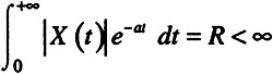
Let X ( t) be a function, or a distribution, with the following property:
| (7.18) | ![]() |
where a is a real and finite constant.
Such a function has a Laplace transform, which is noted either LT[ X ( t)], or more concisely
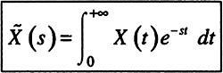
. The Laplace transformation is defined by the integral:
| (7.19) | ![]() |
where the Laplace variable s is usually complex. Writing...