The Finite Element Method for Electromagnetic Modeling

Written by specialists of modeling in electromagnetism, this book provides a comprehensive review of the finite element method for low frequency applications.
In order to present the finite element method, we propose, initially, to implement it on a simple 1D electrostatics example, borrowed from [HOO 89]. We will first formulate this problem in its differential form, then in its variation form. This form of integral will enable us to introduce the concept of first-order finite elements and then second-order finite elements.
We thus consider the problem of Figure 1-1 where two long distant parallel plates of 10m are: one with the electric potential of 0V and the other with the potential of 10V. Between the two plates, the density of electric charges and the dielectric permittivity are assumed to be constant. This problem could represent a hydrocarbon storage tank in which we wish to know the distribution of the electric potential. The lower plate corresponds to the free surface of the liquid, the upper plate to the ceiling of the tank and the intermediate part to the electrically charged vapors.
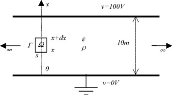
The physical and geometric quantities varying only according to one direction, this problem is 1D in the interval x ? [0, 10] and the electric field E and electric flux density D = ? E vectors have only one non-zero component E x and D x.
Let us consider a parallelepipedic elementary volume of constant section s