Grid Computing for Electromagnetics

Supported with 110+ illustrations, this cutting-edge book clearly describes a high-performance, low-cost method to solving huge numerical electromagnetics problems.
The differential forms of Maxwell's equations in time domain are quite well known to everyone involved in EM research. Nonetheless, it is worth recalling them, as well as their main derivations.
We assume that:
| E = E( r,t) | is the electric field, expressed in V/m. |
| H = H( r,t) | is the magnetic field, expressed in A/m. |
| D = D( r,t) | is the electric flux density vector, expressed in C/m 2. |
| B = B( r,t) | is the magnetic induction, expressed in Wb/m 2. |
| J = J( r,t) | is the electric current density, expressed in A/m 2. |
| ? = ? (r,t) | is the electric charge density, expressed in C/m 3. |
| J m = J m ( r,t) | is the magnetic current density, expressed in V/m 2. |
One of Maxwell's equations is strictly connected with Faraday's law and has the following form:
| (C.1) | 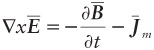 |
The second Maxwell's equation is strictly connected with Ampere's law and has the following form:
| (C.2) | 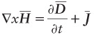 |
From Gauss's Law, we can derive that:
| (C.3) | |
with its dual equation:
| (C.4) | |
It is worth recalling that the magnetic current density is not a physical entity (equivalently, we assume that no magnetic charges can exist).
When dealing with linear, isotropic, and nondispersive (in time and space) materials, the previously mentioned equations are accompanied by the following constitutive equations:
| (C.5) | |
| (C.6) | |
where ?