Microfluid Mechanics: Principles and Modeling
As general probabilistic modeling of physical processes, the DSMC simulation requires the generation of representative values of variables that are distributed in a prescribed manner. This is done through random numbers, which is assumed to be a set of successive random fractions R f and uniformly distributed between 0 and 1. If the probability distribution function (PDF) has a cumulative distribution function (CDF), which can be inversed into an explicit form, the inverse-cumulative method can be applied to sample its representative values; otherwise, the acceptance-rejection method may be used.
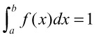
It is assumed that the distribution of variable x may be described by a normalized probability distribution function f( x), and the variable ranges from a to b. The total probability is
| (5A.1) | |
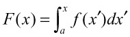
The cumulative distribution function is defined as
| (5A.2) | |
The representative value of x can be sampled by generating a random fraction R f and setting it equal to the cumulative density function F( x) in the form of
| (5A.3) | |
Usually, the value x is obtained through an explicit form of the inverse function F -1( x), if it is possible to invert Eq. (5A.3) to get an explicit function for x.
In the DSMC simulations, there are usually three examples using the inverse-cumulative method to sample the value x.
The variable x is uniformly distributed...