Wind Turbine Control Systems: Principles, Modelling and Gain Scheduling Design

B.4: LPV Descriptions of Nonlinear Systems

B.4 LPV Descriptions of Nonlinear Systems

Although it is possible to find systems governed by the dynamic equations (B.1), in many cases the LPV models are actually nonlinear systems expressed in the form (B.1). In the context of gain scheduling techniques, an LPV model can be interpreted as the family of linear models discussed in the introductory Section B.1. Hence, the first step in the design of a gain-scheduled controller consists precisely in finding an LPV description of the nonlinear or time-varying model. This issue is addressed in this section.

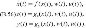
Consider the following nonlinear system


Commonly, there are two approaches to express the nonlinear system (B.56) as an LPV model: one based on classical linearisation and another based on quasi-LPV descriptions.

Linearised LPV Models

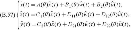
A commonly used method to obtain an LPV description of a nonlinear model is the classic linearisation around the equilibrium or operating points. That is, after linearising the nonlinear model (B.56) we obtain


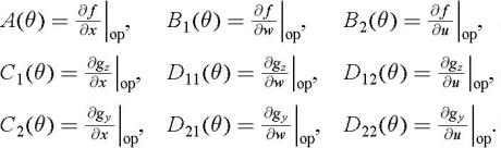
where


The notation op means that the derivatives are evaluated at the operating points parameterised by the variable ?. The operating points of the plant (B.56) are given by the algebraic equation


The expression (B.58) comprises n equations with n + n w + n u unknowns. Therefore, n variables depend on the remaining n w + n u variables denoted by the vector ?.

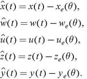
The symbol ^ denotes deviations with respect to the equilibrium values, i.e.,


Note that, in order to implement...

UNLIMITED FREE
ACCESS
TO THE WORLD'S BEST IDEAS

SUBMIT
Already a GlobalSpec user? Log in.

This is embarrasing...

An error occurred while processing the form. Please try again in a few minutes.

Customize Your GlobalSpec Experience

Category: Color Meters and Appearance Instruments
Finish!
Privacy Policy

This is embarrasing...

An error occurred while processing the form. Please try again in a few minutes.