A.1 Scalar Spectral Transport Equation
In the presence of a mean scalar gradient ?? ? and a fluctuating (zero-mean) velocity field u i, the fluctuation field of a passive scalar ? ? with molecular diffusion coefficient ? ? is governed by
| (A.1) |  |
The time-evolutio n equation for the spherically integrated scalar-variance spectrum E ?? ( k, t) obtained from (A.1) can be written as
| (A.2) |  |
where the Schmidt number is defined by
| (A.3) |  |
G ?? is the scalar-variance source term proportional to the uniform mean scalar gradient and the scalar-flux spectrum, and T ?? is the scalar-variance transfer spectrum.
Likewise, the time-evolution equation for the scalar-covariance spectrum E ? ?( k, t) can be written as
| (A.4) |  |
where
| (A.5) | 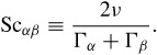 |
G ?? is the corresponding scalar-covariance source term, and T ?? is the scalar-covariance transfer spectrum. In the following, we will relate the SR model for the scalar variance to (A.2); however, analogous expressions can be derived for the scalar covariance from (A.4) by following the same procedure.
A key assumption in deriving the SR model (as well as earlier spectral models; see Batchelor (1959), Saffman (1963), Kraichnan (1968), and Kraichnan (1974)) is that the transfer spectrum is a linear operator with respect to the scalar spectrum (e.g., a linear convection-diffusion model) which has a characteristic time constant that depends only on the velocity spectrum. The linearity assumption (which is consistent with the linear form of (A.1)) ensures...


 TABLE OF CONTENTS