5.1 PLANE STRESS
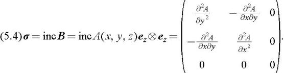
The previously introduced expression for the stress tensor in terms of the Beltrami potential is
Because div inc B = 0, the stress tensor defined in this way automatically satisfies equilibrium.
The Airy stress function solution corresponds to a special form of the Beltrami potential, namely
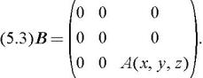
In matrix form with respect to cartesian coordinates this Beltrami tensor is given by
Introducing the stress using the Airy form of the Beltrami potential ensures that the stress tensor satisfies the equilibrium equation div ?=0 and that the corresponding stress state is planar:
The derivation is illustrated in the notebook CQS_airy1.nb :
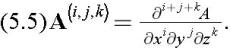
<b class="bold"><< Tensor2Analysis.m</b><b class="bold">SetCoordinates[Cartesian[x, y, z]]</b><b class="bold">B = {{0, 0, 0}, {0, 0, 0}, {0, 0, A [x, y, z]}}</b><b class="bold">(Stress = Inc [B]) // MatrixForm</b><b class="bold">(Div [Stress]) // MatrixForm</b> From now on we use the MATHEMATICA notation for partial differentiation with respect to the arguments, so that, for example
For a stress state to give a solution of the complete system of equations of elasticity, the corresponding strain state must also satisfy the compatibility equations. To compute the strain tensor we require the isotropic compliance tensor, which is constructed as follows:
This allows the strain to be computed from the stress by the double dot product:
We implement the calculations in the form of the MATHEMATICA functions DDot (double dot product) and IsotropicCompliance. For the latter we include an alternative definition of the isotropic compliance tensor as a function of one parameter, nu. This...

 TABLE OF CONTENTS