Elasticity with Mathematica: An Introduction to Continuum Mechanics and Linear Elasticity
Appendix 1: Differential Operators

The solution of physical problems can often be simplified if it is expressed in a particular curvilinear coordinate system instead of the classical cartesian coordinate system.

The mathematical presentation of this subject follows the evolution of ideas as presented in (Malvern, 1969; Soos and Teodosiu, 1983). Our development of programming is built upon the kernel of an existing standard MATHEMATICA package, vectorAnalysis. Our additions and modifications are grouped together in the form of a new package called Tensor2Analaysis.

A.1.1 THE MATHEMATICAL DEFINITIONS

Orthogonal curvilinear coordinate systems

Let us introduce a new system of coordinates ? 1 , ? 2 , ? 3 related to the cartesian coordinates by the functions


We shall assume that the functions can be inverted and possess sufficient smoothness properties. The inverse transformations will be denoted by


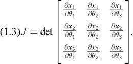
The above smoothness and inversibility hypothesis implies that the Jacobian matrix has a nonvanishing determinant in the domain considered:


A point P in the Euclidean space can be identified by its position vector, denoted by


where i k , k=1, 2, 3 denote the basis vectors of the cartesian system. The point P can be identified either by the cartesian coordinates ( x 1 , x 2 , x 3) or by the curvilinear coordinates ( ? 1 , ? 2 , ? 3).


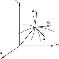
Figure A.1.1: An orthogonal system of coordinates defined by the functions x i( ? ?).

The operators JacobianMatrix and JacobianDeterminant are already...

UNLIMITED FREE
ACCESS
TO THE WORLD'S BEST IDEAS

SUBMIT
Already a GlobalSpec user? Log in.

This is embarrasing...

An error occurred while processing the form. Please try again in a few minutes.

Customize Your GlobalSpec Experience

Category: CMM, Gage, and Inspection Equipment Services
Finish!
Privacy Policy

This is embarrasing...

An error occurred while processing the form. Please try again in a few minutes.