6. The Stokes Equation

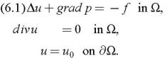
The Stokes equation describes the motion of an incompressible viscous fluid in an n-dimensional domain (with n = 2 or 3):

Here u : ? ? ⁿ is the velocity field and p : ? ? is the pressure. Since we are assuming that the fluid is incompressible, div u = 0 when no sources or sinks are present.

In order for a divergence-free flow to exist with given boundary values u ₀, by Gauss integral theorem we must have

This compatibility condition on u ₀ is obviously satisfied for homogeneous boundary values.

By an appropriate scaling we can assume that the viscosity is 1, which we have already done in writing (6.1).

The given external force field f causes an acceleration of the flow. The pressure gradient gives rise to an additional force which prevents a change in the density. In particular, a large pressure builds up at points where otherwise a source or sink would be created. From a mathematical point of view, the pressure can be regarded as a Lagrange multiplier.

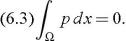
If (6.1) is satisfied for some functions and p ? C ¹( ? ⁾, then we call u and p a classical solution of the Stokes problem. Note that (6.1) only determines the pressure p up to an additive constant, which is usually fixed by enforcing the normalization