7.9 Applications of Integration

Now that we know how to use Integrate and NIntegrate, let's close out this chapter by doing a few examples.

Problem 1: Find the total length of the Lissajous knot parameterized by

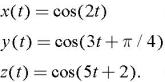
The solution is displayed in Example 7.9.1. We begin by defining the curve parametrically as a position vector, that is, a list of its coordinate functions. Next, just for fun, we plot the curve. The Tube plot style gives a nice effect. In order to find the length of any parameterized curve, we need to integrate the speed, which is the length of the velocity vector. So our next step is to differentiate the position vector, which we do using the "prime" notation for derivative.

In[61]:= (* finding the length of a Lissajous           knot *)         (* define the knot curve *)         <b class="bold">k[</b><i class="emphasis">t</i><b class="bold">_] := {Cos [2</b> <i class="emphasis">t</i><b class="bold">], Cos [3</b> <i class="emphasis">t</i> <b class="bold">+ Pi/4],              Cos [5</b> <i class="emphasis">t</i> <b class="bold">+ 2] };</b>         (* plot the knot *)         <b class="bold">ParametricPlot3D[k[</b>t<b class="bold">], {</b>t<b class="bold">, 0,  2 Pi},            PlotStyle...