Matrix Preconditioning Techniques and Applications

Figures


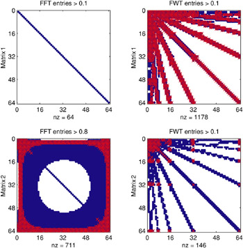
Figure 1.1: Comparison of FFT ( = F AF H) and FWT ( = WAW T ) for compressing two test matrices. Clearly FFT is only good at circulant matrix 1 but FWT is more robust for both examples.

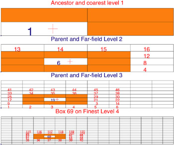
Figure 3.4: The FMM Illustration I of the interaction lists across all levels (for a specified box). Note the parent s near neighbours provide the interaction lists.

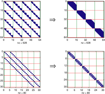
Figure 4.1: Illustration of Lemma 4.1.1 for two examples.

Figure 6.7: Illustration of automatic coarsening by an AMG method, with o/ ?: fine grid points and ?: coarse grid points. (e.g. to produce the right plot, use G=numgrid('A',n); A=delsq(G); lap_lab; xy=[x(:) y(:)]; [C F]=cf_split(A); gplot(A,xy,'bo-'), hold on, gplot(A(C,C),xy(C,:),'ks'))

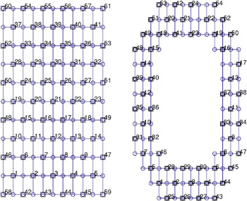
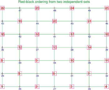
Figure 7.5: Illustration of a red-black ordering (with red in large fonts and black in small fonts, each forming an independent set of nodes). Check with the Mfile multic.m.

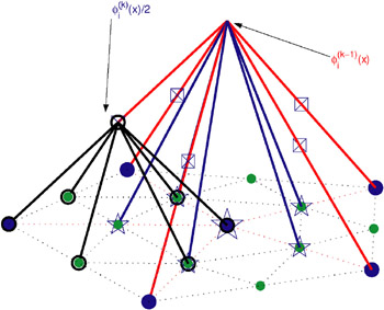
Figure 7.7: Illustration of the fundamental result (7.41) in 2 for the HB basis. Here large ? points are the coarse points and small ? ones are the fine level points. Observe the difference between ( k ) and ( k ?1) the same coarse point (large) ?. The ? (and small ?) points indicate the position of neighbouring ( k )/2.

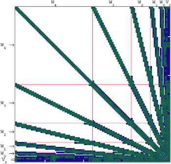
Figure 8.1: Illustration of the finger-like sparsity pattern in a wavelet basis ( J = 5 levels). Recall that V 5 = W 4

UNLIMITED FREE
ACCESS
TO THE WORLD'S BEST IDEAS

SUBMIT
Already a GlobalSpec user? Log in.

This is embarrasing...

An error occurred while processing the form. Please try again in a few minutes.

Customize Your GlobalSpec Experience

Category: Screws
Finish!
Privacy Policy

This is embarrasing...

An error occurred while processing the form. Please try again in a few minutes.