9.5 Reliability Growth
It is common practice, during the development of a system, to make engineering changes as the program develops. These changes are generally made in order to correct design deficiencies and thereby to increase reliability. This elimination of design weakness is known as the reliability growth.
Reliability growth can be characterized by [12]:
-
Expressing the cumulative number of failures as a function of operating time.
-
Expressing failure rate as a function of operating time
-
Expressing mean time between failures as a function of time.
A commonly used reliability growth model is the Duane model [10]. Using data from the development programs of several different and complex equipments, Duane observed that the logarithms of observed cumulative MTBFs,  , was a linear function of time:
| (9.74) | 
|
where  reciprocal of the cumulative MTBF over the observation period of operation [0, t], can be estimated as
We can then also write In H ( t) = - ? In ? + ? In t, from which,
| (9.75) | 
|
which describes a Non-Homogeneous Poisson-Process (NHPP) with Weibull intensity
| (9.76) | 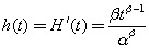
|
The function h( t) has the same functional form of the instantaneous hazard rate of the Weibull distribution. However, while the instantaneous hazard rate is the conditional probability of failure at t + ?t given that there was no failure prior to t (Section 4.5.3), the present intensity function h(t) represents the unconditional probability of failure at time t + ?


 TABLE OF CONTENTS