The time average of a function, u, is denoted by triangular brackets and defined as follows:

(A.1)

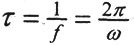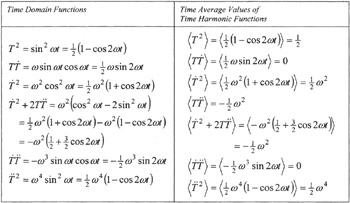
where is the period. Time-average analysis is simplified by neglecting the effects of retardation 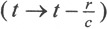. This neglect makes calculations easier but is part of the way in which time average analysis tends to obscure the physical behavior of the electromagnetic fields. Table A.1 presents a variety of time functions relevant to the present analysis of the harmonic dipole and shows the results of the time-averaging process.

Table A.1: Harmonic Time Domain Functions

The radial component of the time-average harmonic Poynting vector is:

(A.2)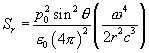

and the angular component of the time average harmonic Poynting vector is:

(A3)

The time average time domain harmonic energy density becomes:

(A.4)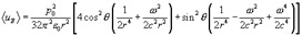

for the electric field energy, and

(A.5)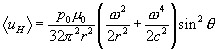

for the magnetic field energy. Expressing these results in terms of wave number 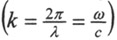, the electric energy density is

(A.6)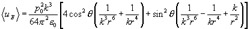

and the magnetic energy density is

(A.7)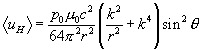

Noting that , the propagating, or radiation, portion of the energy density is

(A.8)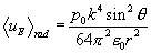

for the electric energy and:

(A.9)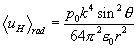

for the magnetic energy. The radiation energy is equally divided between electric and magnetic energy.

The traditional division of energy into propagating radiation energy and fixed reactive energy has a significant conceptual difficulty. Assume the electric field can be broken up into a reactive and radiation term:

(A.10)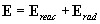

Then, the electric field energy is

(A.11)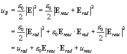

Lumping the cross-term into the reactive field energy leads to the unsatisfying result that the reactive...