6.2.1 Coordinate Transformation

Our first task is to transform the transport equations in Cartesian coordinates to those in curvilinear coordinates. Thus, employing the chain rule, we can write the first-order derivatives as

(6.2)

(6.3)

The next task is to determine derivatives of ?1 and ?2 with respect to x ₁ and x ₂ knowing functions (6.1). To do this, we note that

(6.4)

(6.5)

These relations can be written in matrix form as dx=Ad ?, or

(6.6)

Now, manipulation of Equations 6.4 and 6.5 will show that

(6.7)

(6.8)

where cof denotes cofactor of and Det A stands for determinant of A. Thus, from the last two equations, it is easy to deduce that

(6.9)

(6.10)

(6.11)

(6.12)

where the ?s are called the geometric coefficients and are given by

(6.13)

Further, it follows that

(6.14)

where symbol J stands for the Jacobian of the matrix A. We can now rewrite Equations 6.2 and 6.3 as

(6.15)

(6.16)

6.2.2 Transport Equation

The first task is to transform the general transport equation (5.1) from the ( x ₁, x ₂) coordinate system to the ( ? ₁, ? ₂) coordinate system using relations (6.15) and (6.16). Thus,

(6.17)

This equation can also be written as

(6.18)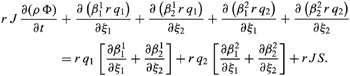

Using definitions (6.13), however, we can show that the terms in the square brackets are identically zero. Hence, Equation 6.18 can be written as

(6.19)

Using...