Introduction to Computational Fluid Dynamics

For advanced undergraduate and first year graduate students in mechanical, aerospace and chemical engineering, this textbook emphasizes understanding CFD through physical principles and examples.
In all the preceding chapters it was shown that discretising the differential transport equations results in a set of algebraic equations of the following form:
| (9.1) | |
where suffix k refers to appropriate neighbouring nodes of node P. In pure conduction problems ( ?= T), A k and S may be functions of T. In the general problem of convective-diffusive transport, ? may stand for any transported variable and A k and S may again be functions of the ? under consideration or any other ? relevant to the system. In curvilinear grid generation, ?= x 1, x 2, and A k and S are again functions of x 1 and x 2. In all such cases, if there are N interior nodes, we need to solve N equations for each variable ? in a prespecified sequence. An iterative solution is particularly attractive when the algebraic equations for different ?s are strongly coupled through coefficients and sources.
In an iterative procedure, convergence implies numerical satisfaction of Equation 9.1 at each interior node for each ?. This satisfaction is checked by the residual in Equation 9.1 at each iteration level 1 (say). Thus
| (9.2) | |
The whole-field convergence is declared when
| (9.3) | 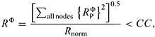 |
where CC stands for the convergence criterion and R norm is a dimensionally correct normalising quantity defined by...