Inverse Problem Theory and Methods for Model Parameter Estimation

When in doubt, smooth.
Sir Harold Jeffreys ( Quoted by Moritz, 1980)
Many inverse problems involve functions: the data set sometimes consists of recordings as a function of time or space, and the main unknown in the parameter set sometimes consists of a function of the spatial coordinates and/or of time.
Quite often, the functions can be approximated by their discretized versions, and an infinite-dimensional problem is then reduced to a finite-dimensional one. In fact, many functions are handled and displayed by digital computers, and their discretization is implicit (like, for instance, when dealing with space images of Earth).
In spite of this, there are situations where the inverse problem is better formulated using functions (i.e., using the concepts of functional analysis). One may go quite far using the functional formulation, even if, at the end, some sort of discretization is used for the actual computations.
Few developments are needed for the general inverse problem (we shall see that the very definition of random function considers successive discretizations). But in the special case where the considered random functions are Gaussian, lots of beautiful mathematics is available that provides efficient methods of resolution.
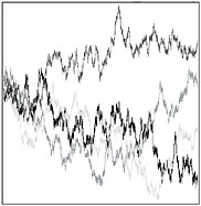
Looking at Figures 5.1 5.2, we can understand what is generally meant by a random function. Each of the figures represents some realizations of the considered random function, each realization being an ordinary function.