6.7 Log-Normal Probability Density

The log-normal probability density is defined by

Figure 6.7 shows some examples of this probability density.

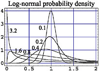Figure 6.7: The log-normal probability density (equation (6.12)). Note that when the dispersion parameter s tends to ? , the probability density tends to the function 1/x, the homogeneous probability density for a Jeffreys quantity.

The log-normal probability density is so called because the logarithm of the variable has a normal (Gaussian) probability density. For the change of variables

transforms f(x) into

with a=s ?, s= ?/ ?, and

In (6.73), the constant ? is often log _e 10, which corresponds to defining x*= log ₁₀ (x/ ?). The constant ? often corresponds to the physical unit used for x (see Example 1.30). Alternatively, the particular choice

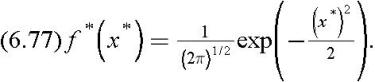
leads to a Gaussian density with zero mean and unit standard deviation:

Figure 6.7 suggests that, for given x ₀, when the dispersion s is very small, the log-normal probability density tends to a Gaussian function. This is indeed the case. For, when s ?0, f(x) takes significant value only in the vicinity of x ₀ , and , i.e.,

If, for given x ₀, the dispersion s is very large, the log-normal probability density tends to a log-uniform probability density (i.e., proportional to 1/ x; see section 1.2.4). For any x not too close to the origin, the argument of the...