Developments in statistical thermodynamics, quantum mechanics, and kinetic theory often require implementation of a spherical coordinate system. Making use of Fig. I.1, we recognize that spherical coordinates can be related to Cartesian coordinates through

and thus

(I.1)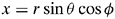

(I.2)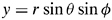

(I.3)

From Eqs. (I.1) and (I.2), we have

(I.4)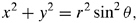

while from Eq. (I.3)

(I.5)

Adding Eqs. (I.4) and (I.5), we obtain, as expected,

(I.6)

Figure I.1: Spherical and Cartesian coordinate systems.

Dividing Eq. (I.4) by Eq. (I.5), we find that

(I.7)

Similarly, dividing Eq. (I.2) by Eq. (I.1), we have

(I.8)

Hence, while Eqs. (I.1), (I.2), and (I.3) express Cartesian coordinates in terms of spherical coordinates, Eqs. (I.6), (I.7), and (I.8) relate spherical coordinates to Cartesian coordinates.

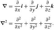
The gradient and Laplacian operators for any orthogonal curvilinear coordinate system ( u ₁, u ₂, u ₃) can be expressed as (Hildebrand, 1962)

(I.9)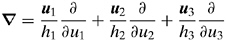

(I.10)

where u _i represents the unit vector for the ith coordinate, with an inherent scale factor given by

(I.11)

The utility of Eqs. (I.9) through (I.11) can be demonstrated by applying them to the familiar Cartesian coordinates, for which

Therefore, using

(I.12)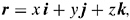

we obtain, from Eq. (I.11),

Subsequently, from Eqs. (I.9) and (I.10), the gradient and Laplacian operators for the Cartesian coordinate system become, as anticipated,

Now, for spherical coordinates, we introduce in a similar fashion,

(I.13)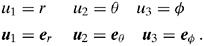

Substituting Eqs. (I.1), (I.2), and (I.3) into Eq. (I.12), we obtain

(I.14)

so that

(I.15)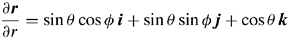

(I.16)

(I.17)

Consequently, from Eq. (I.15),

(I.18)

Similarly, from Eqs.