To compute the Fourier coefficients of a periodic function f of period 1, we multiply f by the functions sin 2 ?kx and cos 2 ?kx (sines and cosines of integer frequencies k). Since the functions sin 2 ? kx and cos 2 ?kx oscillate between +1 and -1, this multiplication produces a function whose graph oscillates between the graphs of + f and - f.

The integral of this product (the area delimited by the graph of the new function) is the Fourier coefficient at a given frequency. The negative area (below the x-axis) is subtracted from the positive area (above the x-axis). We integrate over the period of the function (here, between 0 and 1; for a function periodic of periodic 2 ?, between 0 and 2 ?). Figures 2 5 illustrate this procedure for the function shown in Figure 1.

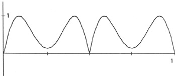Figure 1: The function f( x) = sin(3 sin 2 ?x)

At very high frequencies, the Fourier coefficients of a smooth function tend towards zero. The function changes slowly relative to the rapid, high-frequency oscillations, and these oscillations tend to delimit almost equal amounts of negative and positive areas, producing very small coefficients. But it's not true that Fourier coefficients always get smaller as the frequency increases. For the function shown in Figure 1, the coefficient for cosine of frequency 100, is small (see Figure 4), but...