 The rationale for this handbook is to make adaptive optics technology for
vision science and ophthalmology as broadly accessible as possible. While the
scientific literature chronicles the dramatic recent achievements enabled by
adaptive optics in vision correction and retinal imaging, it does less well at
conveying the practical information required to apply wavefront technology
to the eye. This handbook is intended to equip engineers, scientists, and clinicians
with the basic concepts, engineering tools, and tricks of the trade
required to master adaptive optics-related applications in vision science and
ophthalmology.
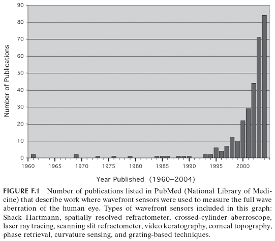
During the past decade, there has been a remarkable expansion of
the application of wavefront-related technologies to the human eye, as
illustrated by the rapidly growing number of publications in this area (shown
in Fig. F.1).
The catalysts for this expansion have been the development of new wavefront
sensors that can rapidly provide accurate and complete descriptions of
the eye’s aberrations, and the demonstration that adaptive optics can provide
better correction of the eye’s aberrations than has previously been possible.
These new tools have generated an intensive effort to revise methods to
correct vision, with the wavefront sensor providing a much needed yardstick
for measuring the optical performance of spectacles, contact lenses, intraocular
lenses, and refractive surgical procedures. Wavefront sensors offer the
promise of a new generation of vision correction methods that can correct
higher order aberrations beyond defocus and astigmatism in cases where
these aberrations significantly blur the retinal image.
The ability of adaptive optics to correct the monochromatic aberrations of
the eye has also created exciting new opportunities to image the normal and
diseased retina at unprecedented spatial resolution. Adaptive optics has
strong roots in astronomy, where it is used to overcome the blurring effects
of atmospheric turbulence, the fundamental limitation on the resolution of
ground-based telescopes. More recently, adaptive optics has found application
in other areas, most notably vision science, where it is used to correct the
eye’s wave aberration. Despite the obvious difference in the scientific objectives
of the astronomy and vision science communities, we share a technology
that is remarkably similar across the two applications.
Recognizing this, together with Jerry Nelson and other colleagues, we
created a center focused on developing adaptive optics technology for both
astronomy and vision science. The Center for Adaptive Optics, with headquarters
at the University of California, Santa Cruz, was founded in 1999 as
a National Science Foundation Science and Technology Center. Initially
under the leadership of Jerry Nelson and more recently of Claire Max, the
Center for Adaptive Optics is a consortium involving more than 30 affiliated
universities, government laboratories, and corporations. The Center has fostered
extensive new collaborations between vision scientists and astronomers
(who very soon discovered they were interested in each others’ science as well
as their technology!). This handbook is a direct result of the Center’s collaborative
energy, with chapters contributed by astronomers and vision scientists
alike.
We wish to thank all of the contributors for generously sharing their expertise,
and even their secrets, within the pages of this book. Especially, we
congratulate Jason Porter, lead editor, and Hope Queener, Julianna Lin,
Karen Thorn, and Abdul Awwal, coeditors, for their tireless dedication to
this significant project.
DAVID R. WILLIAMS
University of Rochester, Rochester, New York
Center for Adaptive Optics
CLAIRE MAX
University of California, Santa Cruz
Center for Adaptive Optics
 TABLE OF CONTENTS