III. H _? Riccati Solution for Augmented Plant Containing Describing Function

The use of the H _? control synthesis procedure presented in Section II will now be demonstrated. This is done for the following system with an unstable plant and a Bang-Bang relay:58

(3.100)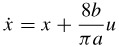

(3.101)

(3.102)

This system is shown in block diagram form in Fig. 3.5 and as a Simulink model in Fig. 3.6.

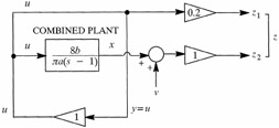Figure 3.5: Block diagram of augmented plant containing a describing function.

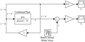Figure 3.6: Simulink model of augmented plant with describing function.

The resulting augmented system in state space form is

(3.103)

The submatrices for the augmented system are

(3.104)

(3.105)

(3.106)

(3.107)

(3.108)

(3.109)

(3.110)

(3.111)

(3.112)

Checking the conditions from Eqs. (3.24 3.28), first note that ( A, B ₂) is stabilizable and ( C ₂, A) is detectable. Secondly,

(3.113)

and

(3.114)

Finally, checking the other rank conditions,

(3.115)

(3.116)

As these conditions are satisfied, the Riccati matrices X and Y can now be determined. From Eqs. (3.38 3.41),56

(3.117)

(3.118)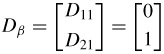

and

(3.119)

(3.120)

The Hamiltonian matrix H _? is derived next:56

(3.121)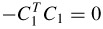

(3.122)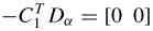

(3.123)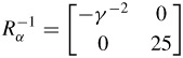

(3.124)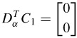

Equation (3.36) gives

(3.125)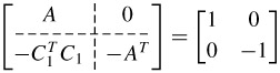

(3.126)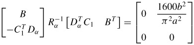

Therefore,

(3.127)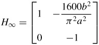

Solving the Riccati Eq. (3.45) gives

(3.128)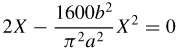

Discarding the trivial solution X = 0 gives

(3.129)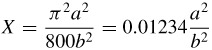

Note that the Riccati equation has degenerated into a Lyapunov equation. Solving for the second Hamiltonian matrix J _? (see Ref. 56),

(3.130)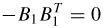

(3.131)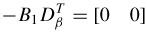

(3.132)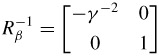

(3.133)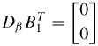

Equation (3.37) gives

(3.134)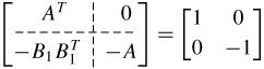

(3.135)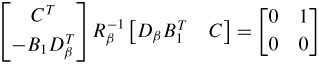

Thus,

(3.136)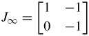

Solving the...