7.2 Root Representation Using the Complex Plane
The roots of Eq. (7.16) were presented in Eq. (7.17) and are repeated here.
These roots can be represented on a complex plane as shown in Fig. 7.9. The complex plane plots the real part of the root on the horizontal axis and the imaginary part of the root on the vertical axis.
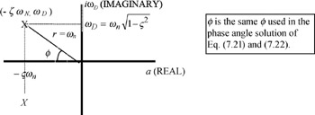 Figure 7.9: Root representation using the complex plane.
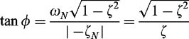
 From trigonometry
so
or
| (7.23) | 
|
It is good to keep ? in units of radians, as we will soon see. Also
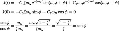
Therefore, if we know ? we can find ? for Eqs. (7.21) and (7.22). This leaves only C 3 to be evaluated. To do this we can assume the initial conditions of x(0) =  , and use Eq. (7.22).
to obtain
Also, we know that
This is the same result as found from the complex plane trigonometry, which proves that the ?s are the same.
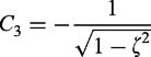
Because C 3 = ?1/sin ? and sin 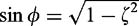 ,
,
Therefore, for an underdamped second-order system with a step input of magnitude y, the time response is
| (7.24) | 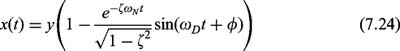
|
This is much nicer than solving for the transient and steady-state solutions and evaluating the constants as in Example 7.2. All we need to determine from the original differential equation is ? n, ?, and y. Radians are compatible units for ? in Eq. (7.24) because ? D t will have units of radians.