Advanced Mathematics For Engineering and Science
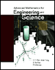
As the product of a close collaboration between two mathematicians and an engineer, this pragmatic text provides the know-how and know-why to understanding mathematics and its many applications.
 TABLE OF CONTENTS
 In Chapter 1, we reviewed several of the standard techniques used to solve ordinary differential equations (O.D.E. s). In particular, we have seen that second order linear differential equations with constant coefficients admit a solution in the form of an exponential function. Since the derivatives of exponential functions are also exponential functions, the differential equation reduces to an algebraic equation [see Equations (1.16 8,9)]. If the coefficients of the differential equation are not constants, then the solution is not of an exponential form. In this chapter, we develop methods of solving O.D.E. s with variable coefficients. As in Chapter 1, we consider second order O.D.E. s. Higher order O.D.E. s can be solved by the same method.
A second order O.D.E. can be written as
| (2.1 1) |  |
where a 2(x) ?0 and ' denotes differentiation with respect to x.
Equation (2.1 1) can be written in standard form as
| (2.1 2a) |  |
where
| (2.1 2b,c,d) |  |
We recall that if b is zero, Equation (2.1 2a) is homogeneous. The solution of Equation (2.1 2a) can be written as
| (2.1 3) |  |
where y h is the homogeneous solution and y p is the particular integral. If b is zero, we have only the homogeneous solution. The particular integral (or particular solution) is usually obtained by the method of variation of parameters which is described in Example 1.18 1 and Section 2.5.
The solution of the homogeneous equation in the neighborhood of a point x 0 is assumed to be given by a power series in (x ?x 0