7.8 NUMERICAL SOLUTION OF ORDINARY DIFFERENTIAL EQUATIONS, INITIAL VALUE PROBLEMS

The order and the degree of an ordinary differential equation (O.D.E.) have been discussed in Chapter 1.

An O.D.E. (or a system of O.D.E. s) with all conditions specified at one value of the independent variable is called an initial value problem. In the case where time is the independent variable, all conditions may be specified at t=0. However if the conditions are specified at more than one point, the O.D.E. with the conditions specified at different points represents a boundary value problem.

For example, the differential equation

(7.8 1)

subject to

(7.8 2a,b)

is a two point boundary value problem whereas if the conditions to be satisfied were

(7.8 2c,d)

it would be an initial value problem.

Similarly

(7.8 3a)

(7.8 3b)

with

(7.8 3c to f)

is an initial value problem of a second order system of differential equations, whereas

(7.8 4a)

(7.8 4b,c)

is a boundary value problem (Sturm-Liouville problem).

In this section, only initial value problems will be considered.

First Order Equations

A first order initial value problem can be written as

(7.8 5a)

(7.8 5b)

Formally integrating Equation (7.8 5a) subject to the initial condition given by Equation (7.8 5b), we obtain

(7.8 6)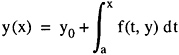

Note that the unknown variable y is inside the integral sign in Equation (7.8 6) and we cannot evaluate such an integral. Equation (7.8 6) is known as an integral equation. We have transformed the differential equation [Equation (7.8 5a)] into an integral equation.

There is a similarity between Equations (7.8 6, 2 20). As...