5.9 DYNAMIC EQUATIONS WITH MULTIPLIERS
The kinematic constraints that describe mechanical joints as well as specified trajectories in the multibody system consisting of interconnected rigid and deformable components can be formulated by using a set of nonlinear algebraic constraint equations. This vector of equations defined by Eq. 134 is shown here for convenience:
| (5.155) | 
|
where  is the vector of linearly independent constraint equations, t is time, and q is the total vector of system generalized coordinates that can be written in a partitioned form as
| (5.156) | 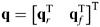
|
where the subscripts r and f refer, respectively, to reference and flexible (elastic) coordinates, and q r and q f are, respectively, the vectors of the system reference and elastic coordinates.
Equation 155 can then be written in terms of reference and elastic coordinates as follows:
| (5.157) | 
|
In the following q f represents the vector of generalized elastic coordinates that can be introduced by using the finite-element method, Rayleigh Ritz methods, or a set of experimentally identified data (Shabana 1986). This vector can be a set of physical or modal elastic coordinates.
Using Eq. 133a, the general system differential equations of motion of the multibody system can be written in a matrix form as
| (5.158) | 
|
where M and K are, respectively, the system mass and stiffness matrices, C q is the constraint Jacobian matrix, ? is the vector of Lagrange multipliers, Q e is the vector of generalized externally applied forces, and


 TABLE OF CONTENTS