We calculate the capacitance of two parallel wires that are shown in Figure D-1. The radius of each wire is a.

Figure D-1: Equipotential contours surrounding two line charges + ? _? and - ? _?. The surfaces at r = a are equipotential surfaces, therefore the electric field will always be normal to the metal surfaces.

The two wires can be replaced with two line charges + ? _? and - ? _?. The precise location of these equivalent line charges is determined from the requirement that the surfaces of the metal wires be equipotential surfaces. This implies that the tangential electric fields will always be equal to zero on these surfaces. The potential V( x, y) at the point P is given by

(D.1)

The plane at the midpoint between the two wires is an equipotential surface that is equal to zero potential. Other equipotential contours are found by setting

(D.2)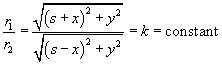

This can be written as

(D.3)

or

(D.4)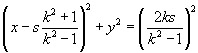

The common factor

has been added to both sides of (D.3) in order to complete the squares. Equation (D.4) is an equation for a family of circles that have radii

(D.5)

and are centered at the points

(D.6)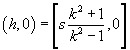

where

Eliminating the term s between (D.5) and (D.6), we obtain

(D.7)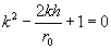

The two solutions for this equation are given by

(D.8)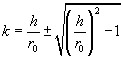

The root k with the + sign will give the equipotential contours in the region x >...