Mathematical Methods in Chemical Engineering

In this section we consider two examples. In the first we simply develop the successive approximations without concern for their domain of validity, while in the second we also examine this aspect.
For the linear ODE
with IC
construct the solution by successive approximations.
The analytic solution is readily obtained as
and let us now develop the successive approximations.
The function f( x, y) = y is continuous and satisfies the Lipschitz condition (with K = 1 + ?, where ? > 0) for
= { x ?( ? ?, ?)}. The successive approximations are given by
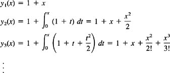
Thus we have
and
Taking the limit as n ? ? yields
as expected.
For the ODE
with IC
construct the successive approximations, and find the largest range of x for the solution.
The analytic solution can again be obtained easily by separation of variables:
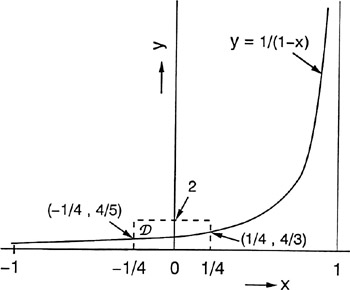
which is clearly continuous for ? ? < x < 1, a range that contains the initial value of x (i.e., x = 0). A plot of eq. (2.5.8) is shown in Figure 2.3.
The nonlinear function f( x, y) = y 2 is continuous for all x and y. It also satisfies the Lipschitz condition for all y, since
so that max[2 y +