I INITIAL VALUE PROBLEMS 3.1: DEFINITIONS, LINEARITY, AND SUPERPOSITION

A general nth-order linear ordinary differential equation (ODE) can be written as

where the coefficients a _j( x) are continuous over the closed interval x ? [ a, b], and a ₀( x) ? 0 for x ? [ a, b]. If f( x) = 0, eq. (3.1.1) is said to be homogeneous; otherwise it is nonhomogeneous.

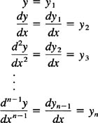
If we denote

then from eq. (3.1.1) we have

Thus the nth-oder ODE (3.1.1) reduces to a set of n coupled first-order ODEs of the form

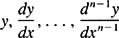
We recall from chapter 2 that, when the ICs are provided, unique solutions of nonlinear equations of the form (3.1.2) are guaranteed to exist if the f _j have continuous partial derivatives with respect to all y _j. For the linear problem at hand, with the mild restrictions on a _j( x) given above, the latter is ensured. Thus a unique solution for the ODE (3.1.1) exists for all x ? [ a, b], provided that the values of

are given at some point x ₀ ? [ a, b].

Although we have used the term linear above, in connection with eq. (3.1.1), let us define what is meant by linearity of a differential operator. Consider

Then L[ y] is linear if

where c ₁ and c ₂ are constants.